1. Introduction
The first lesson in the NVIDIA DLI — Generative AI exam prep series will equip you with a solid PyTorch foundation. This is the primary framework used throughout the entire DLI course, from Diffusion Models to Large Language Models (LLMs).
In the NVIDIA DLI assessment, you will write code directly — not multiple-choice questions. Therefore, mastering the basic patterns of PyTorch is a prerequisite.
Exam tip: The NVIDIA DLI assessment requires you to write and debug PyTorch code directly. Make sure you can write a training loop, nn.Module, and perform tensor operations without referring to documentation.
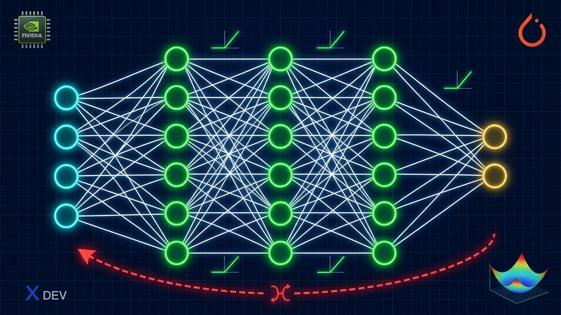
2. PyTorch Tensors & Autograd
2.1 Tensor Basics
Tensor is the core data structure of PyTorch — similar to NumPy arrays but capable of running on GPU and supporting automatic differentiation.
import torch

# Create tensor from list
x = torch.tensor([1.0, 2.0, 3.0])

# Create tensor with specific shape
zeros = torch.zeros(3, 4)          # shape: (3, 4)
ones = torch.ones(2, 3, 4)         # shape: (2, 3, 4)
rand = torch.randn(64, 3, 32, 32)  # batch of 64 RGB 32x32 images

# Check shape and dtype
print(rand.shape)   # torch.Size([64, 3, 32, 32])
print(rand.dtype)   # torch.float32
print(rand.device)  # cpu
2.2 Tensor Operations & Broadcasting
PyTorch supports broadcasting similar to NumPy — allowing operations between tensors with different shapes.
# Reshape operations
x = torch.randn(2, 3, 4)
y = x.view(2, 12)        # reshape to (2, 12)
z = x.permute(0, 2, 1)   # swap dims: (2, 4, 3)
w = x.unsqueeze(0)        # add dim: (1, 2, 3, 4)

# Matrix multiplication
a = torch.randn(3, 4)
b = torch.randn(4, 5)
c = a @ b                 # shape: (3, 5)
# or: c = torch.matmul(a, b)

# Broadcasting
x = torch.randn(64, 256)  # (batch, features)
bias = torch.randn(256)   # (features,)
result = x + bias          # bias is broadcast: (64, 256)
| Operation | Syntax | Notes |
|---|---|---|
| Reshape | x.view() / x.reshape() | view requires contiguous memory |
| Transpose | x.permute() / x.T | permute is more flexible for multiple dims |
| Add dim | x.unsqueeze(dim) | Commonly used to prepare for broadcasting |
| Remove dim | x.squeeze(dim) | Removes dim with size = 1 |
| Matrix mul | a @ b | Equivalent to torch.matmul |
| Concat | torch.cat([a, b], dim=0) | Concatenate along specified dim |
2.3 Autograd — Automatic Differentiation
Autograd is PyTorch's automatic gradient computation system. When you set requires_grad=True, PyTorch tracks all operations on that tensor and builds a computational graph.
# Basic autograd
x = torch.tensor([2.0, 3.0], requires_grad=True)
y = x ** 2 + 3 * x       # y = x² + 3x
loss = y.sum()            # scalar output
loss.backward()           # compute gradient

print(x.grad)  # dy/dx = 2x + 3 → tensor([7., 9.])
Computational Graph:

  x (requires_grad=True)
  │
  ├──→ x ** 2 ──→ + ──→ y ──→ sum() ──→ loss
  │                ↑                        │
  └──→ 3 * x ─────┘                   backward()
                                            │
                                       x.grad = 2x + 3
Exam tip: In the DLI assessment, you may encounter the error "trying to backward through the graph a second time". Solution: use
loss.backward(retain_graph=True)or recompute the forward pass. This is a very common error during the assessment.
3. nn.Module & Building Networks
3.1 nn.Module Pattern
Every neural network in PyTorch inherits from nn.Module. This is a pattern you must memorize:
import torch.nn as nn

class SimpleNet(nn.Module):
    def __init__(self, input_dim, hidden_dim, output_dim):
        super().__init__()  # MUST call super().__init__()
        self.fc1 = nn.Linear(input_dim, hidden_dim)
        self.relu = nn.ReLU()
        self.fc2 = nn.Linear(hidden_dim, output_dim)

    def forward(self, x):
        x = self.fc1(x)
        x = self.relu(x)
        x = self.fc2(x)
        return x

# Usage
model = SimpleNet(784, 256, 10)
x = torch.randn(32, 784)  # batch of 32
output = model(x)          # shape: (32, 10)
3.2 Common Layers
| Layer | Purpose | Key Params |
|---|---|---|
nn.Linear(in, out) | Fully connected layer | in_features, out_features |
nn.Conv2d(in_ch, out_ch, k) | 2D convolution | in_channels, out_channels, kernel_size |
nn.BatchNorm2d(ch) | Batch normalization | num_features |
nn.GroupNorm(g, ch) | Group normalization | num_groups, num_channels |
nn.ReLU() | Activation function | inplace (optional) |
nn.Dropout(p) | Regularization | p = drop probability |
nn.Embedding(V, D) | Token embedding | num_embeddings, embedding_dim |
3.3 nn.Sequential — Quick Models
For simple models, you can use nn.Sequential instead of creating a class:
# Quick approach with nn.Sequential
model = nn.Sequential(
    nn.Linear(784, 256),
    nn.ReLU(),
    nn.Dropout(0.2),
    nn.Linear(256, 128),
    nn.ReLU(),
    nn.Linear(128, 10)
)

# Inspect model
print(model)
# Count parameters
total_params = sum(p.numel() for p in model.parameters())
print(f"Total params: {total_params:,}")
3.4 Code: MLP for MNIST
import torch
import torch.nn as nn
from torchvision import datasets, transforms

# Data
transform = transforms.Compose([
    transforms.ToTensor(),
    transforms.Normalize((0.1307,), (0.3081,))
])
train_data = datasets.MNIST('./data', train=True, download=True,
                            transform=transform)
train_loader = torch.utils.data.DataLoader(train_data, batch_size=64,
                                           shuffle=True)

# Model
class MNISTClassifier(nn.Module):
    def __init__(self):
        super().__init__()
        self.flatten = nn.Flatten()
        self.layers = nn.Sequential(
            nn.Linear(28 * 28, 512),
            nn.ReLU(),
            nn.Dropout(0.2),
            nn.Linear(512, 256),
            nn.ReLU(),
            nn.Dropout(0.2),
            nn.Linear(256, 10)
        )

    def forward(self, x):
        x = self.flatten(x)   # (B, 1, 28, 28) → (B, 784)
        return self.layers(x)  # (B, 784) → (B, 10)
4. Training Loop Pattern
4.1 Loss Functions
| Loss Function | Use Case | Input shape |
|---|---|---|
nn.CrossEntropyLoss() | Multi-class classification | logits (B, C), labels (B,) |
nn.MSELoss() | Regression, diffusion noise prediction | (B, *) vs (B, *) |
nn.BCEWithLogitsLoss() | Binary / multi-label classification | logits (B, C), labels (B, C) |
nn.L1Loss() | Regression (robust to outliers) | (B, *) vs (B, *) |
Exam tip:
nn.CrossEntropyLossalready includes softmax internally — do NOT add softmax to the output layer. This is a mistake many people make in the assessment.nn.MSELosswill be very important when you learn Diffusion Models (predict noise).
4.2 Optimizers
# SGD — basic, manually manage learning rate
optimizer = torch.optim.SGD(model.parameters(), lr=0.01, momentum=0.9)

# Adam — most popular, adaptive learning rate
optimizer = torch.optim.Adam(model.parameters(), lr=1e-3)

# AdamW — Adam + proper weight decay (used for Transformers)
optimizer = torch.optim.AdamW(model.parameters(), lr=1e-4, weight_decay=0.01)
| Optimizer | When to Use | Characteristics |
|---|---|---|
| SGD | CNNs, when fine-grained control is needed | Requires careful lr tuning, add momentum |
| Adam | Default for most tasks | Fast convergence, minimal tuning needed |
| AdamW | Transformers, LLMs, Diffusion | Decoupled weight decay, more correct than Adam |
4.3 Full Training Loop
This is the most important pattern — you must be able to write a complete training loop in the assessment:
import torch
import torch.nn as nn

# Setup
device = torch.device('cuda' if torch.cuda.is_available() else 'cpu')
model = MNISTClassifier().to(device)
criterion = nn.CrossEntropyLoss()
optimizer = torch.optim.Adam(model.parameters(), lr=1e-3)

# Training loop
num_epochs = 10
for epoch in range(num_epochs):
    model.train()  # ENABLE training mode (dropout, batchnorm active)
    total_loss = 0

    for batch_idx, (images, labels) in enumerate(train_loader):
        images, labels = images.to(device), labels.to(device)

        # Forward pass
        outputs = model(images)
        loss = criterion(outputs, labels)

        # Backward pass
        optimizer.zero_grad()  # IMPORTANT: reset gradients
        loss.backward()        # compute gradients
        optimizer.step()       # update weights

        total_loss += loss.item()

    avg_loss = total_loss / len(train_loader)
    print(f"Epoch [{epoch+1}/{num_epochs}], Loss: {avg_loss:.4f}")

# Evaluation
model.eval()  # DISABLE dropout, batchnorm uses running stats
with torch.no_grad():  # DO NOT compute gradients → save memory
    correct = 0
    total = 0
    for images, labels in test_loader:
        images, labels = images.to(device), labels.to(device)
        outputs = model(images)
        _, predicted = torch.max(outputs, 1)
        total += labels.size(0)
        correct += (predicted == labels).sum().item()

    print(f"Accuracy: {100 * correct / total:.2f}%")
Training Loop Flow:

  ┌─────────────────────────────────────────────┐
  │              FOR EACH EPOCH                  │
  │  ┌────────────────────────────────────────┐  │
  │  │         FOR EACH BATCH                 │  │
  │  │                                        │  │
  │  │  1. images, labels = batch.to(device)  │  │
  │  │              │                         │  │
  │  │  2. outputs = model(images)   FORWARD  │  │
  │  │              │                         │  │
  │  │  3. loss = criterion(outputs, labels)  │  │
  │  │              │                         │  │
  │  │  4. optimizer.zero_grad()     RESET    │  │
  │  │              │                         │  │
  │  │  5. loss.backward()          BACKWARD  │  │
  │  │              │                         │  │
  │  │  6. optimizer.step()          UPDATE   │  │
  │  │              │                         │  │
  │  └──────────────┼─────────────────────────┘  │
  │                 ▼                             │
  │         Next Epoch                            │
  └─────────────────────────────────────────────┘
Exam tip: The order
zero_grad() → backward() → step()is MANDATORY. Forgettingzero_grad()will cause gradients to accumulate across batches — this is bug #1 in the DLI assessment. Always remembermodel.train()before training andmodel.eval()+torch.no_grad()before evaluation.
4.4 GPU Acceleration
# Check GPU
print(torch.cuda.is_available())        # True/False
print(torch.cuda.device_count())        # Number of GPUs
print(torch.cuda.get_device_name(0))    # GPU name

# Move model and data to GPU
device = torch.device('cuda' if torch.cuda.is_available() else 'cpu')
model = model.to(device)

# IN training loop — data must also be on the same device
images = images.to(device)
labels = labels.to(device)
Exam tip: Common error: model is on GPU but data is still on CPU (or vice versa). PyTorch will throw "Expected all tensors to be on the same device". Always ensure model and data are on the same
device.
5. CNN Architecture
5.1 Convolutional Layers
Convolution slides a kernel (filter) across the input image to extract features. Each kernel detects a specific pattern (edges, textures, shapes).
# Basic Conv2d
conv = nn.Conv2d(
    in_channels=3,    # RGB input
    out_channels=32,  # 32 filters → 32 feature maps
    kernel_size=3,    # 3×3 kernel
    stride=1,         # step size
    padding=1          # zero-padding to preserve spatial size
)

# Output shape calculation:
# H_out = (H_in + 2*padding - kernel_size) / stride + 1
# Example: (32 + 2*1 - 3) / 1 + 1 = 32 (size preserved)
Convolution Operation:

Input (3 channels)          Kernel (3×3)         Output (1 feature map)
┌─────────────┐            ┌───────┐              ┌──────────┐
│ ■ ■ ■ ■ ■ ■│   ×        │ w w w │     =        │ ○ ○ ○ ○  │
│ ■ ■ ■ ■ ■ ■│            │ w w w │              │ ○ ○ ○ ○  │
│ ■ ■ ■ ■ ■ ■│            │ w w w │              │ ○ ○ ○ ○  │
│ ■ ■ ■ ■ ■ ■│            └───────┘              │ ○ ○ ○ ○  │
│ ■ ■ ■ ■ ■ ■│                                   └──────────┘
│ ■ ■ ■ ■ ■ ■│         32 kernels → 32 feature maps
└─────────────┘

Shape flow: (B, 3, 32, 32) → Conv2d(3, 32, 3, padding=1) → (B, 32, 32, 32)
5.2 Pooling Layers
Pooling reduces spatial dimensions, helping reduce computation and increase receptive field:
| Pooling | How It Works | When to Use |
|---|---|---|
nn.MaxPool2d(2) | Takes max value within each 2×2 window | Feature detection, standard CNNs |
nn.AvgPool2d(2) | Takes average within each 2×2 window | Smoother features |
nn.AdaptiveAvgPool2d((1,1)) | Pools to fixed size regardless of input | Before fully-connected layer |
5.3 Batch Normalization vs Group Normalization
This knowledge is extremely important for the Diffusion Models section in later lessons.
| Property | BatchNorm | GroupNorm |
|---|---|---|
| Normalizes across | Batch dimension (N) | Channel groups (C/G) |
| Depends on batch size | Yes — noisy with small batches | No — works well with any batch size |
| Training vs Inference | Different (running stats) | Same |
| Commonly used in | Traditional CNNs (ResNet) | Diffusion Models, small groups |
| Syntax | nn.BatchNorm2d(C) | nn.GroupNorm(G, C) |
# BatchNorm — normalize across batch
bn = nn.BatchNorm2d(64)         # 64 channels

# GroupNorm — normalize within groups of channels
gn = nn.GroupNorm(
    num_groups=32,    # split 64 channels into 32 groups (2 ch/group)
    num_channels=64
)

# Both accept input shape: (B, C, H, W)
x = torch.randn(8, 64, 16, 16)
print(bn(x).shape)  # (8, 64, 16, 16)
print(gn(x).shape)  # (8, 64, 16, 16)
BatchNorm vs GroupNorm:

BatchNorm: normalize along ↓ (batch axis)    GroupNorm: normalize along → (channel groups)
┌────────────────────────┐                    ┌────────────────────────┐
│  Sample 1: [c1 c2 c3 c4]│                    │  Sample 1: [c1 c2│c3 c4]│
│  Sample 2: [c1 c2 c3 c4]│  ← normalize      │            group1│group2 │ ← normalize
│  Sample 3: [c1 c2 c3 c4]│    each column     │                  │       │   each group
│  Sample 4: [c1 c2 c3 c4]│                    │  Sample 2: [c1 c2│c3 c4]│
└────────────────────────┘                    └────────────────────────┘

→ Diffusion Models use GroupNorm because batch_size is usually small
  and noise levels vary → BatchNorm statistics are unstable
Exam tip: When building U-Net for Diffusion Models (later lessons), you will always use GroupNorm instead of BatchNorm. Reason: diffusion training typically uses small batch sizes, and each sample has a different noise level → BatchNorm statistics become noisy. Remember the rule: Diffusion = GroupNorm.
5.4 Code: Simple CNN for Image Classification
class SimpleCNN(nn.Module):
    def __init__(self, num_classes=10):
        super().__init__()

        # Conv Block 1: (B, 1, 28, 28) → (B, 32, 14, 14)
        self.block1 = nn.Sequential(
            nn.Conv2d(1, 32, kernel_size=3, padding=1),
            nn.BatchNorm2d(32),
            nn.ReLU(),
            nn.MaxPool2d(2)
        )

        # Conv Block 2: (B, 32, 14, 14) → (B, 64, 7, 7)
        self.block2 = nn.Sequential(
            nn.Conv2d(32, 64, kernel_size=3, padding=1),
            nn.BatchNorm2d(64),
            nn.ReLU(),
            nn.MaxPool2d(2)
        )

        # Conv Block 3: (B, 64, 7, 7) → (B, 128, 1, 1)
        self.block3 = nn.Sequential(
            nn.Conv2d(64, 128, kernel_size=3, padding=1),
            nn.BatchNorm2d(128),
            nn.ReLU(),
            nn.AdaptiveAvgPool2d((1, 1))  # global average pooling
        )

        # Classifier
        self.classifier = nn.Linear(128, num_classes)

    def forward(self, x):
        x = self.block1(x)     # (B, 32, 14, 14)
        x = self.block2(x)     # (B, 64, 7, 7)
        x = self.block3(x)     # (B, 128, 1, 1)
        x = x.view(x.size(0), -1)  # (B, 128)
        x = self.classifier(x)     # (B, 10)
        return x
CNN Architecture Flow:

Input: (B, 1, 28, 28)
         │
    ┌────▼────────────────────────┐
    │ Conv2d(1→32, 3×3, pad=1)   │
    │ BatchNorm2d(32)             │  Block 1
    │ ReLU                        │
    │ MaxPool2d(2)                │
    └────┬────────────────────────┘
         │ (B, 32, 14, 14)
    ┌────▼────────────────────────┐
    │ Conv2d(32→64, 3×3, pad=1)  │
    │ BatchNorm2d(64)             │  Block 2
    │ ReLU                        │
    │ MaxPool2d(2)                │
    └────┬────────────────────────┘
         │ (B, 64, 7, 7)
    ┌────▼────────────────────────┐
    │ Conv2d(64→128, 3×3, pad=1) │
    │ BatchNorm2d(128)            │  Block 3
    │ ReLU                        │
    │ AdaptiveAvgPool2d(1,1)      │
    └────┬────────────────────────┘
         │ (B, 128, 1, 1)
    ┌────▼────────────────────────┐
    │ Flatten → (B, 128)          │
    │ Linear(128, 10)             │  Classifier
    └────┬────────────────────────┘
         │ (B, 10)
         ▼
      Output logits
6. Cheat Sheet
| Concept | Code Pattern | Remember |
|---|---|---|
| Create model | class MyModel(nn.Module) | Always call super().__init__() |
| Forward pass | output = model(x) | Call model as function, don't call .forward() directly |
| Training mode | model.train() | Enables dropout, batchnorm training stats |
| Eval mode | model.eval() + torch.no_grad() | Disables dropout, uses running stats |
| Training loop | zero_grad → forward → loss → backward → step | Order is CRITICAL |
| GPU transfer | .to(device) | Both model AND data |
| Classification loss | nn.CrossEntropyLoss() | Already includes softmax |
| Diffusion loss | nn.MSELoss() | Predict noise, compute MSE |
| Diffusion norm | nn.GroupNorm(G, C) | Independent of batch size |
| Transformer optimizer | AdamW | Proper weight decay |
7. Practice Questions
The following questions simulate the NVIDIA DLI coding assessment style — you need to read code, find bugs, and write complete code.
Q1: Fix the broken training loop
The code below has a bug that prevents the model from converging. Find and fix the error:
for epoch in range(10):
    model.train()
    for images, labels in train_loader:
        images, labels = images.to(device), labels.to(device)
        outputs = model(images)
        loss = criterion(outputs, labels)
        loss.backward()
        optimizer.step()
Show Answer Q1
Bug: Missing optimizer.zero_grad() before loss.backward(). Not resetting gradients causes them to accumulate across batches, preventing the model from converging or converging incorrectly.
for epoch in range(10):
    model.train()
    for images, labels in train_loader:
        images, labels = images.to(device), labels.to(device)
        outputs = model(images)
        loss = criterion(outputs, labels)

        optimizer.zero_grad()  # ← ADD THIS LINE
        loss.backward()
        optimizer.step()
Standard order: zero_grad() → backward() → step(). In practice, zero_grad() can be placed before forward as well, but it MUST come before backward().
Q2: Implement a 3-layer CNN
Write a CNN class that takes RGB images (3, 64, 64) and outputs 5 classes. Requirements:
- 3 convolutional blocks, each block: Conv2d → BatchNorm2d → ReLU → MaxPool2d(2)
- Channels: 3 → 32 → 64 → 128
- End with AdaptiveAvgPool2d + Linear
Show Answer Q2
class ThreeLayerCNN(nn.Module):
    def __init__(self, num_classes=5):
        super().__init__()
        self.features = nn.Sequential(
            # Block 1: (B, 3, 64, 64) → (B, 32, 32, 32)
            nn.Conv2d(3, 32, kernel_size=3, padding=1),
            nn.BatchNorm2d(32),
            nn.ReLU(),
            nn.MaxPool2d(2),

            # Block 2: (B, 32, 32, 32) → (B, 64, 16, 16)
            nn.Conv2d(32, 64, kernel_size=3, padding=1),
            nn.BatchNorm2d(64),
            nn.ReLU(),
            nn.MaxPool2d(2),

            # Block 3: (B, 64, 16, 16) → (B, 128, 8, 8)
            nn.Conv2d(64, 128, kernel_size=3, padding=1),
            nn.BatchNorm2d(128),
            nn.ReLU(),
            nn.MaxPool2d(2),
        )
        self.pool = nn.AdaptiveAvgPool2d((1, 1))
        self.classifier = nn.Linear(128, num_classes)

    def forward(self, x):
        x = self.features(x)        # (B, 128, 8, 8)
        x = self.pool(x)            # (B, 128, 1, 1)
        x = x.view(x.size(0), -1)   # (B, 128)
        x = self.classifier(x)      # (B, 5)
        return x

# Verify
model = ThreeLayerCNN(num_classes=5)
x = torch.randn(4, 3, 64, 64)
print(model(x).shape)  # torch.Size([4, 5])
Q3: Trace tensor shapes through a network
Given the model below and input shape (8, 1, 32, 32). Record the shape at each step:
model = nn.Sequential(
    nn.Conv2d(1, 16, kernel_size=5, stride=2, padding=2),  # Step A
    nn.ReLU(),
    nn.Conv2d(16, 32, kernel_size=3, stride=1, padding=0), # Step B
    nn.ReLU(),
    nn.AdaptiveAvgPool2d((4, 4)),                           # Step C
    nn.Flatten(),                                            # Step D
    nn.Linear(32 * 4 * 4, 10),                              # Step E
)
Show Answer Q3
Output size formula: H_out = (H_in + 2*padding - kernel_size) / stride + 1
Input:  (8, 1, 32, 32)

Step A: Conv2d(1, 16, k=5, s=2, p=2)
        H = (32 + 2*2 - 5) / 2 + 1 = 16
        → (8, 16, 16, 16)

Step B: Conv2d(16, 32, k=3, s=1, p=0)
        H = (16 + 2*0 - 3) / 1 + 1 = 14
        → (8, 32, 14, 14)

Step C: AdaptiveAvgPool2d((4, 4))
        → (8, 32, 4, 4)

Step D: Flatten()
        → (8, 512)       # 32 * 4 * 4 = 512

Step E: Linear(512, 10)
        → (8, 10)
Key insight: AdaptiveAvgPool2d always outputs a fixed size regardless of input — very useful when input size can vary.
Q4: GroupNorm vs BatchNorm — when to use which?
You are building a U-Net for a Diffusion Model. Each block has Conv2d → ??? → SiLU. Which normalization do you choose and why? Write code for one block.
Show Answer Q4
Choose GroupNorm. Reasons:
- Small batch size: Diffusion training typically uses batch size 1-8 because images are large → BatchNorm statistics are too noisy
- Different noise levels: Each sample in the batch has a different timestep (noise level) → normalizing across the batch is not appropriate
- Inference consistency: GroupNorm behaves the same during training and inference
class DiffusionBlock(nn.Module):
    def __init__(self, in_channels, out_channels, num_groups=32):
        super().__init__()
        self.conv = nn.Conv2d(in_channels, out_channels,
                              kernel_size=3, padding=1)
        self.norm = nn.GroupNorm(num_groups, out_channels)
        self.act = nn.SiLU()  # SiLU is more common than ReLU in diffusion

    def forward(self, x):
        x = self.conv(x)
        x = self.norm(x)
        x = self.act(x)
        return x

# Example usage
block = DiffusionBlock(64, 128, num_groups=32)
x = torch.randn(2, 64, 32, 32)  # batch_size = 2, small!
print(block(x).shape)  # (2, 128, 32, 32)
Rule: In all Diffusion architectures (U-Net, DiT), always use nn.GroupNorm. Activation is typically nn.SiLU() (Swish) instead of ReLU.
Q5: Debug gradient issue — detach() vs torch.no_grad()
What's wrong with the code below? The output of feature_extractor should not have gradients (freeze backbone), but classifier still needs to be trained.
feature_extractor = pretrained_model.features
classifier = nn.Linear(512, 10).to(device)
optimizer = torch.optim.Adam(classifier.parameters(), lr=1e-3)

for images, labels in train_loader:
    images, labels = images.to(device), labels.to(device)

    # Extract features (should be frozen)
    with torch.no_grad():
        features = feature_extractor(images)

    # Classify
    outputs = classifier(features)
    loss = criterion(outputs, labels)

    optimizer.zero_grad()
    loss.backward()    # ← Is there a problem?
    optimizer.step()
Show Answer Q5
Issue: This code actually works correctly for this case! torch.no_grad() prevents gradient computation for feature_extractor, and the features tensor will not have requires_grad. Gradients still flow through classifier normally.
However, there are 2 approaches and you need to understand the difference:
# Approach 1: torch.no_grad() — DO NOT compute gradients, save memory
with torch.no_grad():
    features = feature_extractor(images)
# features.requires_grad = False
# Gradient DOES NOT flow back through feature_extractor
# ✅ Use when you want to fully freeze and save GPU memory

# Approach 2: .detach() — detach tensor from computational graph
features = feature_extractor(images).detach()
# features.requires_grad = False
# Feature extractor STILL computes forward (memory used for graph)
# but gradient is cut at .detach()
# ⚠️ Less efficient because graph is built then cut

# Approach 3: Freeze parameters — most common approach
for param in feature_extractor.parameters():
    param.requires_grad = False
# ✅ Most explicit, commonly used in fine-tuning
| Approach | Gradient flow | Memory | When to use |
|---|---|---|---|
torch.no_grad() | No graph computed | Most efficient | Inference, frozen features |
.detach() | Cut at detach point | More expensive | When partial gradient flow is needed |
| Freeze params | Weights not updated | Still builds graph | Explicit fine-tuning |
8. Conclusion
Lesson 1 has equipped you with all the PyTorch fundamentals needed for the NVIDIA DLI Generative AI course. Make sure you can:
- Write a complete training loop without referring to documentation
- Create an nn.Module class with
__init__andforward - Trace tensor shapes through each layer
- Distinguish GroupNorm vs BatchNorm — especially important for Diffusion Models
- Debug common errors: missing
zero_grad(), device mismatch, gradient issues
Next lesson: Lesson 2 — Transformer Architecture & Attention Mechanism — the foundation for Transformers and LLMs.