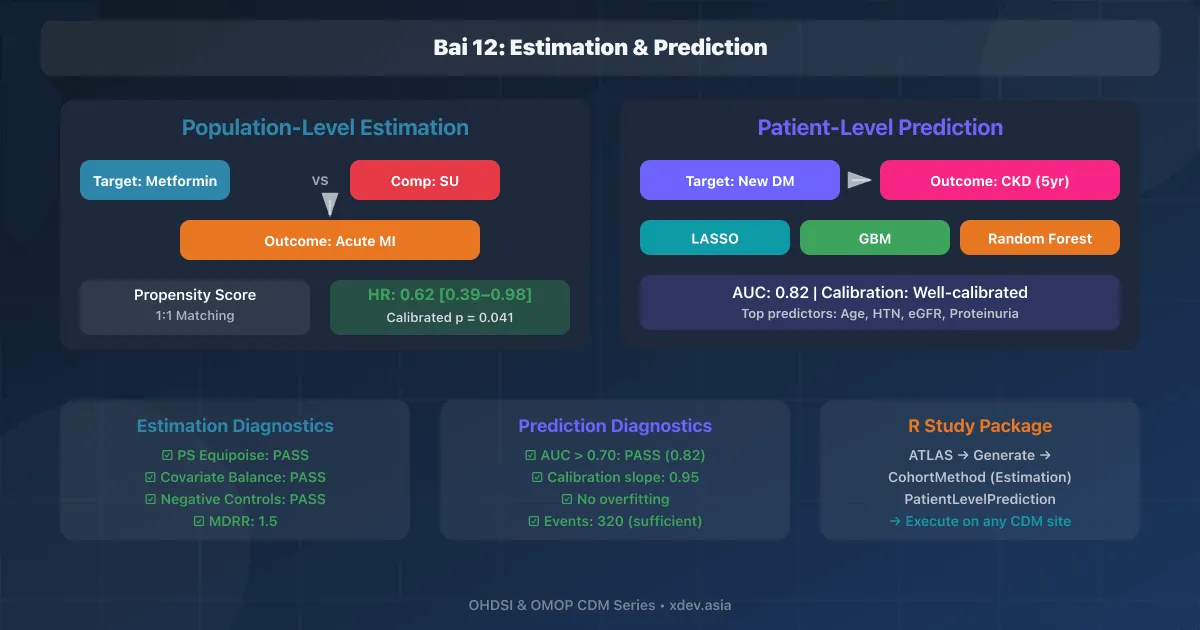
はじめに
この記事では、ATLAS の最も高度な分析機能のうち 2 つに焦点を当てます。
- 集団レベル効果推定 (PLE): 集団レベルでの薬の有効性/副作用を推定します。
- 患者レベル予測 (PLP): 各患者に発生する転帰の確率を予測します。
1. 人口レベルの効果推定 (PLE)
1.1 問題
Câu hỏi: "Thuốc A có làm GIẢM/TĂNG nguy cơ [outcome]
          so với thuốc B không?"

Ví dụ thực tế:
  T (Treatment): Metformin (thuốc ĐTĐ)
  C (Comparator): Sulfonylurea (thuốc ĐTĐ khác)
  O (Outcome): Nhồi máu cơ tim (MI)

  → Metformin có giảm nguy cơ MI so với SU không?
1.2 ATLAS での設計
ATLAS → Estimation → New Estimation

┌─────────────────────────────────────────────────────────┐
│  Estimation: Metformin vs SU — MI Risk                  │
│                                                         │
│  Comparisons:                                           │
│  ┌───────────────────────────────────────────┐          │
│  │  Target: [New Metformin Users ▼]          │          │
│  │  Comparator: [New Sulfonylurea Users ▼]   │          │
│  └───────────────────────────────────────────┘          │
│                                                         │
│  Outcomes:                                              │
│  ☑ Acute Myocardial Infarction                         │
│  ☑ Stroke (thêm outcome phụ)                           │
│                                                         │
│  Analysis Settings:                                     │
│  ☑ Propensity Score Matching (1:1)                      │
│  ☑ Propensity Score Stratification (5 strata)           │
│  ☑ Inverse Probability of Treatment Weighting           │
│                                                         │
│  Negative Controls:                                     │
│  ☑ Import negative control concepts (50 outcomes)       │
│                                                         │
│  [▶ Generate R Package]                                 │
└─────────────────────────────────────────────────────────┘
1.3 新規ユーザーのコホート設計
Tại sao "New User"?
─────────────────────
Tránh prevalent user bias:

Timeline (Sai):
  Patient đã dùng Metformin 2 năm → bắt đầu theo dõi
  → Bias: BN dung nạp tốt mới còn dùng → sống sót tốt hơn

Timeline (Đúng — New User):
  Lần đầu dùng Metformin ─────────→ theo dõi
       ↑ Index date

Điều kiện New User cohort:
  1. Lần đầu dùng thuốc (no prior 365 days)
  2. Có ≥365 ngày observation trước index date
  3. Không có prior outcome
1.4 傾向スコア
Propensity Score = P(nhận Treatment | covariates)

Mục đích: Cân bằng confounders giữa 2 nhóm
         (vì đây KHÔNG phải RCT)

Covariates ATLAS tự trích xuất:
  - Demographics (age, gender, race)
  - Conditions (trước 365 ngày)
  - Drugs (trước 365 ngày)
  - Procedures, Measurements
  - Visit count
  → Hàng nghìn covariates tự động

Matching 1:1:
┌─────────────────┐     ┌─────────────────┐
│ Metformin Users │     │ SU Users        │
│ PS = 0.72       │────→│ PS = 0.73       │  ← matched
│ PS = 0.45       │────→│ PS = 0.44       │  ← matched
│ PS = 0.88       │  ✗  │ (no match)      │  ← excluded
│ PS = 0.31       │────→│ PS = 0.30       │  ← matched
└─────────────────┘     └─────────────────┘

→ After matching: 2 nhóm tương đồng về covariates
→ Kiểm tra SMD < 0.1 cho tất cả features
1.5 ネガティブコントロールの結果
Negative Control = Outcome mà thuốc KHÔNG có tác dụng

Mục đích: Phát hiện systematic bias

Ví dụ negative controls cho Metformin vs SU:
  - Gãy xương cẳng tay (fracture)
  - Viêm ruột thừa (appendicitis)
  - Điếc (hearing loss)
  → Thuốc đái tháo đường KHÔNG ảnh hưởng các outcome này

Kết quả mong đợi:
  Negative control HR ≈ 1.0

Nếu negative controls cho HR ≠ 1.0 hệ thống:
  → CÓ residual bias → cần calibrate p-value
Empirical Calibration:
                    ●
              ●    ●  ●
          ●  ●  ● ● ●●  ●
     ─────●──●●●●●●─●──●──────── HR = 1.0
           ● ●  ●● ●● ●
              ●   ●  ●
                   ●

Nếu negative controls lệch: p-value cần calibrate
  UnCalibrated p = 0.03
  Calibrated p   = 0.12 → KHÔNG còn có ý nghĩa!
2. 患者レベルの予測 (PLP)
2.1 問題
Câu hỏi: "Bệnh nhân X có xác suất bao nhiêu sẽ phát
          triển [outcome] trong [time window]?"

Ví dụ:
  Target: BN Type 2 DM mới chẩn đoán
  Outcome: Chronic Kidney Disease (CKD)
  Time-at-risk: 5 năm

  → Model dự đoán: BN này có 23% nguy cơ CKD
                    trong 5 năm tới
2.2 ATLAS での設計
ATLAS → Prediction → New Prediction

┌─────────────────────────────────────────────────────────┐
│  Prediction: CKD Risk in DM Patients                    │
│                                                         │
│  Target Cohort:                                         │
│  [New-Onset Type 2 DM ▼]                               │
│                                                         │
│  Outcome Cohort:                                        │
│  [Chronic Kidney Disease ▼]                             │
│                                                         │
│  Time-at-risk:                                          │
│  Start: Cohort start + [1] day                          │
│  End:   Cohort start + [1825] days (5 years)            │
│                                                         │
│  Models:                                                │
│  ☑ LASSO Logistic Regression                            │
│  ☑ Gradient Boosting Machine                            │
│  ☑ Random Forest                                        │
│                                                         │
│  Covariates:                                            │
│  ☑ Demographics                                         │
│  ☑ Conditions (prior 365d, prior 30d)                   │
│  ☑ Drugs (prior 365d)                                   │
│  ☑ Measurements (prior 365d)                            │
│  ☑ Procedures (prior 365d)                              │
│                                                         │
│  [▶ Generate R Package]                                 │
└─────────────────────────────────────────────────────────┘
2.3 相互検証プロセス
Dữ liệu CDM (10,000 BN Type 2 DM)
     │
     ├── 75% Training (7,500)
     │     │
     │     ├── Fold 1: Train 5,625 / Val 1,875
     │     ├── Fold 2: Train 5,625 / Val 1,875
     │     └── Fold 3: Train 5,625 / Val 1,875
     │
     └── 25% Test (2,500) — KHÔNG bao giờ dùng khi train

→ 3-fold cross-validation trên Training set
→ Đánh giá final trên Test set
2.4 モデルの評価
Discrimination (AUC-ROC):
  ┌─────────────────────────────┐
  │ 1.0 ──────────────── ●      │
  │      ╱               │      │
  │     ╱       AUC=0.82 │      │
  │    ╱        ─────     │      │
  │   ╱ ╱             ╱  │      │
  │  ╱╱         ╱╱╱      │      │
  │ ╱     ╱╱╱            │      │
  │╱╱╱                   │      │
  0───────────────────────1     │
  └─────────────────────────────┘
  AUC > 0.80: Tốt (acceptable for clinical use)
  AUC > 0.90: Rất tốt

Calibration:
  ┌─────────────────────────────┐
  │ Observed                    │
  │ 0.5 ●                      │
  │      ╱●                    │
  │     ╱  ●      ← Trên đường │
  │    ╱ ●   ●      45° = tốt  │
  │   ╱●                       │
  │  ●                         │
  │ ╱                           │
  0───────────── 0.5            │
  │    Predicted                │
  └─────────────────────────────┘
  Predicted 20% → thực tế ~20% xảy ra → well-calibrated
2.5 結果 — 上位の予測因子
LASSO Logistic Regression — Top Predictors:

┌────┬──────────────────────────────────┬─────────┐
│ #  │ Predictor                        │ Coeff   │
├────┼──────────────────────────────────┼─────────┤
│  1 │ Age ≥ 65                         │ +0.82   │
│  2 │ Hypertension (prior 365d)        │ +0.65   │
│  3 │ eGFR < 60 (prior measurement)   │ +0.58   │
│  4 │ Proteinuria (prior 365d)         │ +0.52   │
│  5 │ ACE inhibitor use               │ +0.38   │
│  6 │ HbA1c > 9% (prior measurement)  │ +0.35   │
│  7 │ Obesity                          │ +0.28   │
│  8 │ Heart failure (prior 365d)       │ +0.25   │
│  9 │ Female gender                    │ −0.12   │
│ 10 │ Statin use                       │ −0.18   │
└────┴──────────────────────────────────┴─────────┘

→ Age, HTN, eGFR thấp, protein niệu: predictor mạnh nhất
→ Statin use: protective effect nhẹ
3. R スタディ パッケージを生成する
3.1 ATLAS からのエクスポート
ATLAS → Estimation/Prediction → [Analysis name] → Utilities

Download R Package:
  estimation-metformin-vs-su/
  ├── DESCRIPTION
  ├── NAMESPACE
  ├── R/
  │   ├── Main.R
  │   ├── Diagnostics.R
  │   └── Export.R
  ├── inst/
  │   ├── settings/
  │   │   ├── TCosCohortDefinitions.json
  │   │   ├── NegativeControlOutcomes.csv
  │   │   └── analysisSettings.json
  │   └── sql/
  │       └── CreateCohorts.sql
  └── extras/
      └── CodeToRun.R
3.2 スタディパッケージの実行
# extras/CodeToRun.R

library(DatabaseConnector)
library(CohortMethod)  # cho Estimation
# hoặc library(PatientLevelPrediction)  # cho Prediction

# Connection details
connectionDetails <- createConnectionDetails(
  dbms = "postgresql",
  server = "localhost/ohdsi",
  user = "ohdsi_app",
  password = keyring::key_get("ohdsi"),
  port = 5432
)

# CDM schema info
cdmDatabaseSchema <- "cdm"
cohortDatabaseSchema <- "results"
cohortTable <- "estimation_cohort"

# Output folder
outputFolder <- "output/metformin_vs_su"

# Execute study
execute(
  connectionDetails = connectionDetails,
  cdmDatabaseSchema = cdmDatabaseSchema,
  cohortDatabaseSchema = cohortDatabaseSchema,
  cohortTable = cohortTable,
  outputFolder = outputFolder,
  createCohorts = TRUE,
  synthesizePositiveControls = TRUE,
  runAnalyses = TRUE,
  runDiagnostics = TRUE,
  maxCores = 4
)
3.3 PLE の結果
Hazard Ratio Results:
┌─────────────────────────────────────────────────────┐
│ Target: Metformin (N=3,200)                         │
│ Comparator: Sulfonylurea (N=3,200)                  │
│ Outcome: Acute MI                                   │
│                                                     │
│ Method: PS Matching 1:1                              │
│ Matched pairs: 2,850                                 │
│                                                     │
│ Events Target: 28 (0.98%)                            │
│ Events Compar: 45 (1.58%)                            │
│                                                     │
│ Calibrated HR: 0.62 [95% CI: 0.39 - 0.98]           │
│ Calibrated p:  0.041                                 │
│                                                     │
│ → Metformin giảm 38% nguy cơ MI so với SU            │
│ → Kết quả có ý nghĩa thống kê (p < 0.05)            │
│                                                     │
│ ⚠ Diagnostics:                                      │
│   PS equipoise: PASS (preference score overlap)      │
│   Covariate balance: PASS (all SMD < 0.1)            │
│   Negative controls: PASS (centered around HR=1)     │
│   MDRR: 1.5 (minimum detectable relative risk)       │
└─────────────────────────────────────────────────────┘
4. 診断と品質評価
4.1 推定診断
Trước khi tin kết quả Estimation, kiểm tra:

1. Preference Score Distribution
   ─────────────────────────────
   Metformin:  ▁▂▃▅▇██▇▅▃▂▁
   SU:         ▁▂▃▅▇██▇▅▃▂▁
   → Cần overlap đáng kể (equipoise)
   → Nếu không overlap: confounding by indication

2. Covariate Balance (after matching)
   ────────────────────────────────────
   Before: 150 covariates có SMD > 0.1
   After:    0 covariates có SMD > 0.1
   → PASS

3. Kaplan-Meier Plot
   ───────────────────
   1.0 ┬────────────────────────
       │ ──── Metformin
       │ ─ ─ SU
   0.98│──────────────
       │     ── ──     ──────── Metformin (higher survival)
   0.96│          ── ──
       │               ── ── ── SU
   0.94│
       └────────────────────────
       0     1     2     3  years

4. Negative Control Plot
   ───────────────────────
   Systematic error: mean = 0.02, SD = 0.08
   → Acceptable (mean ≈ 0, SD < 0.2)
4.2 予測診断
PLP Diagnostics checklist:
  ☑ AUC > 0.70 (minimum acceptable)
  ☑ Calibration slope ∈ [0.8, 1.2]
  ☑ Calibration intercept ∈ [-0.2, 0.2]
  ☑ Brier score < baseline
  ☑ No overfitting (train AUC ≈ test AUC)
  ☑ Sufficient outcome events (≥100)
  ☑ Adequate sample size (events per variable > 10)
概要
| 特長 | 入力 | 出力 | アプリケーション |
|---|---|---|---|
| 見積もり | ターゲット vs 比較対象 → 結果 | ハザード比 + CI | 薬の有効性・安全性を比較 |
| 予測 | 目標 → 結果 (時間枠) | 患者ごとのリスクスコア | 個人のリスクを予測する |
| PS マッチング | 共変量 | バランスの取れたコホート | 交絡を減らす |
| ネガティブコントロール | 既知のヌル効果 | 経験的校正 | 系統的な偏りの検出 |
次の記事: ACHILLES — データの特性評価とソース プロファイリング