
ATLAS handles "cohort definition" and basic "characterization". When you need advanced statistical methods (causal inference, ML), you need HADES — the official OHDSI R package suite. This article gives you the stack overview, the PLE/PLP workflow, and how to publish a network study.
1. What HADES is

40+ R packages, MIT-licensed, installable from CRAN or GitHub.
2. Installation
# Install Strategus (orchestrator) - pulls in the other packages
install.packages("Strategus")

# Or install individually
install.packages(c(
  "DatabaseConnector", "SqlRender", "FeatureExtraction",
  "CohortMethod", "PatientLevelPrediction", "Characterization",
  "CohortDiagnostics", "Achilles", "DataQualityDashboard"
))

# JDBC driver for Postgres
DatabaseConnector::downloadJdbcDrivers("postgresql")
Requirements: R >= 4.2, Java >= 11, 16 GB+ RAM for 1M+ person datasets.
3. Connecting to the database
library(DatabaseConnector)
connectionDetails <- createConnectionDetails(
  dbms = "postgresql",
  server = "host/db_name",
  user = "omop_reader",
  password = Sys.getenv("OMOP_PASSWORD"),
  port = 5432,
  pathToDriver = "~/jdbcDrivers"
)

cdmDatabaseSchema <- "cdm"
cohortDatabaseSchema <- "results"
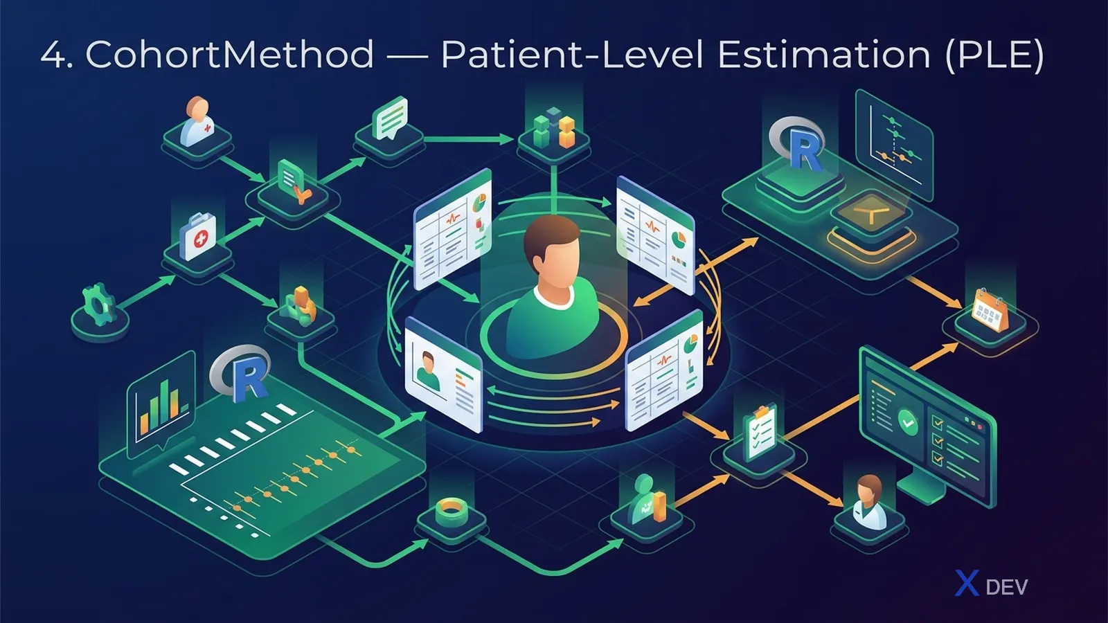
4. CohortMethod — Patient-Level Estimation (PLE)
PLE answers: "Drug A vs. Drug B — which causes fewer side effects of type X?" Comparative effectiveness research.
4.1 PLE workflow
library(CohortMethod)

# 1. Extract data
cmData <- getDbCohortMethodData(
  connectionDetails = connectionDetails,
  cdmDatabaseSchema = cdmDatabaseSchema,
  targetId = 1,         # Cohort A id
  comparatorId = 2,     # Cohort B id
  outcomeIds = c(3),    # Outcome cohort
  covariateSettings = createDefaultCovariateSettings()
)

# 2. Propensity score model
ps <- createPs(
  cohortMethodData = cmData,
  prior = createPrior("laplace", exclude = c(0))
)

# 3. Match 1:1 nearest neighbor
strataPop <- matchOnPs(ps, maxRatio = 1)

# 4. Outcome model (Cox)
outcomeModel <- fitOutcomeModel(
  population = strataPop,
  modelType = "cox",
  stratified = TRUE
)

summary(outcomeModel)
# Hazard Ratio: 0.85 (95% CI 0.78-0.93)
4.2 OHDSI standard diagnostics
Before trusting any result, check:
- Equipoise: sufficient PS overlap between the two cohorts
- Covariate balance: SMD < 0.1 for every covariate after matching
- Negative-control distribution: HR for negative controls should be near 1
- Empirical calibration: adjust HR for systematic error
OHDSI standard: only publish results that pass every diagnostic.
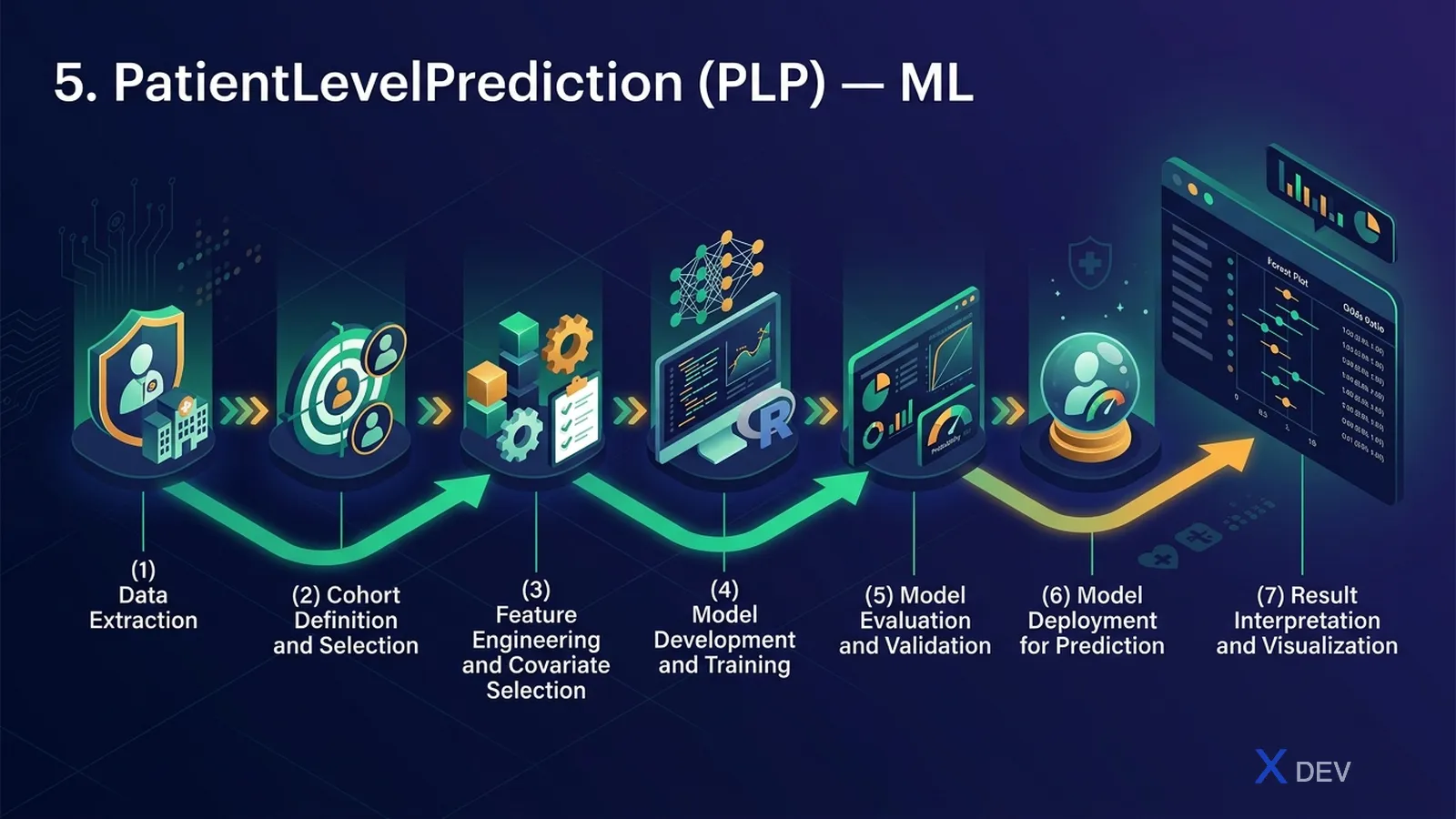
5. PatientLevelPrediction (PLP) — ML
PLP answers: "What is the probability that patient X develops Y in the next T days?"
5.1 PLP code
library(PatientLevelPrediction)

# 1. Get plpData
plpData <- getPlpData(
  databaseDetails = createDatabaseDetails(...),
  covariateSettings = createDefaultCovariateSettings(),
  cohortId = 1,    # at-risk population
  outcomeIds = 2,  # outcome
  ...
)

# 2. Population
population <- createStudyPopulation(
  plpData = plpData,
  outcomeId = 2,
  riskWindowStart = 1,
  riskWindowEnd = 365,
  requireTimeAtRisk = TRUE
)

# 3. Train Lasso
modelSettings <- setLassoLogisticRegression()
results <- runPlp(
  plpData = plpData,
  population = population,
  modelSettings = modelSettings,
  splitSettings = createDefaultSplitSetting(splitSeed = 42)
)

# 4. View
viewPlp(results)
# AUC = 0.78, calibration intercept = -0.05
5.2 External validation
External validation = run a model trained on CDM A → predict on CDM B (same schema, different data). This is gold for clinical ML — it proves the model generalizes.
externalValidatePlp(
  plpResult = results,
  validationDatabaseDetails = list(otherCdmDetails)
)
6. Characterization (advanced cohort comparison)
library(Characterization)

# Setup
cSettings <- createCharacterizationSettings(
  timeAtRiskSettings = createTimeAtRiskSettings(
    riskWindowStart = 1, riskWindowEnd = 365
  ),
  dechallengeRechallengeSettings = createDechallengeRechallengeSettings(
    targetIds = c(1, 2),
    outcomeIds = c(3)
  ),
  aggregateCovariateSettings = createAggregateCovariateSettings(
    targetIds = c(1, 2), outcomeIds = c(3)
  )
)

runCharacterizationAnalyses(
  connectionDetails = connectionDetails,
  cdmDatabaseSchema = cdmDatabaseSchema,
  characterizationSettings = cSettings,
  outputDirectory = "char_results/"
)
Outputs: time-to-event, dechallenge-rechallenge (drug-event causality), aggregate covariates for cohort A vs. B.
7. SelfControlledCaseSeries (SCCS)
A method for situations without a comparator group — patients act as their own control (comparing exposed periods to unexposed periods). Suitable for pharmacovigilance of rarely used drugs.
library(SelfControlledCaseSeries)

sccsData <- getDbSccsData(
  connectionDetails = connectionDetails,
  cdmDatabaseSchema = cdmDatabaseSchema,
  outcomeIds = c(3),
  exposureIds = c(1)
)

sccsModel <- fitSccsModel(...)
8. Strategus — orchestrating multiple methods
Strategus is JSON config + an R workflow that runs the entire pipeline (DQ → CohortDiagnostics → PLE → PLP → Char) for a single study.
library(Strategus)

# 1. Define modules
analysisSpecifications <- createEmptyAnalysisSpecificiations() %>%
  addCharacterizationModuleSpecifications(...) %>%
  addCohortMethodModuleSpecifications(...) %>%
  addPatientLevelPredictionModuleSpecifications(...)

# 2. Run on local CDM
execute(
  analysisSpecifications = analysisSpecifications,
  executionSettings = createCdmExecutionSettings(
    workDatabaseSchema = "results",
    cdmDatabaseSchema = "cdm",
    workFolder = "tmp/work",
    resultsFolder = "tmp/results"
  )
)
Output uses a common schema → upload to a central server for meta-analysis.
9. Network studies pattern

Vietnam can join as a Site — you do not need advanced coding skills, just a CDM and the ability to run an R package.
10. EvidenceSynthesis (meta-analysis)
When you have results from N sites:
library(EvidenceSynthesis)

# Input: per-site HR + log SE
results <- data.frame(
  site = c("VN", "EU1", "EU2", "US1"),
  logRr = c(-0.16, -0.20, -0.18, -0.22),
  seLogRr = c(0.05, 0.04, 0.03, 0.02)
)

# Random-effects meta-analysis
meta <- computeBayesianMetaAnalysis(results)
plotMetaAnalysisForest(meta, results)
11. Common HADES pitfalls
- ❌ Skipping negative controls → systematic bias goes uncorrected
- ❌ Training PLP without external validation → undetected overfitting
- ❌ Excluding key confounders from the PS model → bias
- ❌ Overlap between target and comparator cohorts → strong bias
- ❌ Not checking covariate balance after matching → meaningless analysis
- ❌ Test set leakage from feature extraction → falsely high AUC
12. HADES documentation
- Book of OHDSI chapters 12-15 (PLE, PLP, SCCS, network studies)
- HADES website: ohdsi.github.io/Hades/
- OHDSI Forum: forums.ohdsi.org
- Strategus tutorial videos
- Case studies on Atlas Demo
13. Learning roadmap for HADES
- Learn OMOP SQL and ATLAS (1 month)
- R + tidyverse basics (2 weeks)
- CohortDiagnostics — run diagnostics on one cohort (1 week)
- CohortMethod tutorial on Eunomia (2 weeks)
- PatientLevelPrediction tutorial (2 weeks)
- Join one network study as a contributor (1-2 months)
- Lead a small study (3-6 months)
14. Vietnam use cases
| Question | Method |
|---|---|
| Which hypertension treatment strategy works best for Vietnamese patients? | CohortMethod (PLE) |
| Predict which diabetic patients will be readmitted | PatientLevelPrediction (PLP) |
| Compare cancer epidemiology with Western data | Characterization |
| Monitor side effects of newly approved drugs | SelfControlledCaseSeries |
| Join a DARWIN EU study | Strategus + share aggregate results |
Conclusion
HADES turns the CDM into a full RWE laboratory. Investing in HADES = investing in becoming a real OHDSI Practitioner. Vietnam has a big opportunity to participate in network studies via EHDEN/DARWIN/N3C.
Next article: Production OMOP — Postgres tuning, partitioning, security.