Introduction
Neural Networks are the foundation of all modern AI — from image recognition models to ChatGPT. You can think of a neural network as a decision factory: data comes in → goes through many processing steps → output.
This lesson builds understanding from the bottom up: starting with a single "worker" (neuron), then assembling it into a "team" (network), and finally teaching the team how to "improve" (backpropagation).
import numpy as np
import matplotlib.pyplot as plt

np.random.seed(42)
1. Perceptron: From Biology to Mathematics
1.1 Biological neurons — Inspiration for AI
The human brain has ~86 billion neurons. Each neuron acts as a simple decision maker:
- Get information via dendrites (multiple inputs — like hearing opinions from multiple sources)
- Treatment in cell body/soma (consider all opinions)
- Signal through axon if sufficient stimulation (makes decision: "yes" or "no")
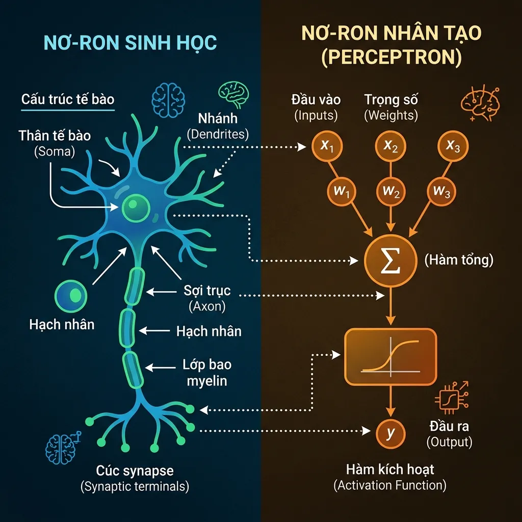
Real life example: Imagine you're deciding whether to go out to dinner with friends:
| Factor (input) | Importance level (weight) | Today's Situation |
|---|---|---|
| Got money? | w₁ = 0.4 (important) | x₁ = 1 (yes) |
| Is it nice weather? | w₂ = 0.1 (less important) | x₂ = 0 (rain) |
| Are you going, buddy? | w₃ = 0.5 (very important) | x₃ = 1 (yes) |
Total score: 0.4×1 + 0.1×0 + 0.5×1 = 0.9 → Exceed the threshold of 0.5 → GO! 🎉
1.2 Perceptron — Artificial Neuron (1958)
Frank Rosenblatt modeled the neuron into a mathematical formula:
z = w₁x₁ + w₂x₂ + ... + wₙxₙ + b = W·x + b
ŷ = f(z)    # f là activation function — quyết định "bắn" hay "không"
Look familiar? This is the dot product from the previous post + an activation function!
class Perceptron:
    def __init__(self, n_inputs, learning_rate=0.1):
        # Khởi tạo trọng số ngẫu nhiên nhỏ
        self.weights = np.random.randn(n_inputs) * 0.01
        self.bias = 0.0
        self.lr = learning_rate

    def predict(self, x):
        z = np.dot(x, self.weights) + self.bias
        return 1 if z >= 0 else 0  # Step function: ≥0 → "có", <0 → "không"

    def train(self, X, y, epochs=100):
        for epoch in range(epochs):
            errors = 0
            for xi, yi in zip(X, y):
                ypred = self.predict(xi)
                error = yi - ypred
                # Perceptron update rule: sai → điều chỉnh trọng số
                self.weights += self.lr * error * xi
                self.bias    += self.lr * error
                errors += abs(error)
            if errors == 0:
                print(f"Converged at epoch {epoch}")
                break

# === Bài toán AND ===
# AND: chỉ cho 1 khi CẢ HAI input = 1
X_and = np.array([[0,0],[0,1],[1,0],[1,1]])
y_and = np.array([0, 0, 0, 1])

p = Perceptron(n_inputs=2)
p.train(X_and, y_and, epochs=50)
print("AND predictions:", [p.predict(x) for x in X_and])  # [0, 0, 0, 1] ✅
print(f"Trọng số học được: w={p.weights}, b={p.bias:.2f}")
💡 Exercise 1.2:
- Train the Perceptron for the OR problem (x₁=0,x₂=0→0; x₁=0,x₂=1→1; x₁=1,x₂=0→1; x₁=1,x₂=1→1). How many epochs does it converge?
- Draw the decision boundary that the perceptron has learned. Hint: it's located
w₁x₁ + w₂x₂ + b = 0.
1.3 Limits of Single Perceptron — XOR Problem
The single perceptron only classifies linear data — meaning it can only draw a straight line to divide the data.
AND: có thể chia bằng 1 đường thẳng ✅     XOR: KHÔNG thể chia ❌
          x₂                                      x₂
     1  | 0   1                               1  | 1   0
        |  ╱                                      |
     0  | 0 ╱ 0                               0  | 0   1
        +--------                                 +--------
          0   1   x₁                               0   1   x₁
XOR: (0,0)→0, (0,1)→1, (1,0)→1, (1,1)→0 → There is no divisible line!
Solution: Arrange multiple perceptrons into multiple layers → Multilayer Perceptron (MLP). Each layer "draws" a dividing line, many layers work together → can draw any curve.
💡 Exercise 1.3: Try training a Single Perceptron for the XOR problem. Does it converge? What is the final error?
2. Activation Functions — "Activation Threshold"
Why do we need an activation function?
Normal life example: If each class is only multiplication and addition (linear), then even if you stack 1000 classes, it will still only be 1 class — because consecutive multiplication = 1 larger multiplication:
y = W₃(W₂(W₁x + b₁) + b₂) + b₃ = (W₃W₂W₁)x + ... = W'x + b'
→ 3 lớp linear = 1 lớp linear to hơn! Vô nghĩa!
Activation functions create non-linearity — like you're not just "considering" but also "interesting" or "rejecting" each decision step.
2.1 Common activation functions
def sigmoid(x):
    """Nén mọi input vào khoảng (0, 1) — giống "xác suất" """
    return 1 / (1 + np.exp(-np.clip(x, -500, 500)))

def sigmoid_derivative(x):
    s = sigmoid(x)
    return s * (1 - s)

def tanh(x):
    """Nén vào (-1, 1) — zero-centered, tốt hơn sigmoid"""
    return np.tanh(x)

def relu(x):
    """ReLU: giữ nguyên nếu dương, bỏ nếu âm — đơn giản mà hiệu quả"""
    return np.maximum(0, x)

def relu_derivative(x):
    return (x > 0).astype(float)

def gelu(x):
    """GELU: smooth version of ReLU — dùng trong GPT, BERT"""
    return 0.5 * x * (1 + np.tanh(np.sqrt(2/np.pi) * (x + 0.044715 * x**3)))

def leaky_relu(x, alpha=0.01):
    """Leaky ReLU: giống ReLU nhưng không "giết chết" neuron âm"""
    return np.where(x > 0, x, alpha * x)
2.2 Comparison — When to use what?
| Activation | Range | Advantages | Problem | Where to use |
|---|---|---|---|---|
| Sigmoid | (0, 1) | Output is the same as probability | Vanishing gradient | Output layer (binary) |
| Tanh | (-1, 1) | Zero-centered | Vanishing gradient | Hidden layers (RNN) |
| ReLU | [0, ∞) | Fast calculation, no vanishing | Dying ReLU (neurons die permanently) | Hidden layers (CNN, MLP) |
| Leaky ReLU | (-∞, ∞) | Fix dying neurons | Add hyperparameter α | Hidden layers |
| GELU | Smooth | Smooth, natural | Slightly expensive | Transformers (BERT, GPT) |
| SiLU/Swish | Smooth | Good for deep networks | Expensive | LLaMA, PaLM |
Rule of thumb:
- Working on Transformer/LLM? → use GELU
- Working on CNN/MLP regular? → use ReLU
- Output layer classification? → use Sigmoid (2 layers) or Softmax (multi-layer)
💡 Exercise 2:
- Draw a graph of 4 activation functions (Sigmoid, Tanh, ReLU, GELU) on the same figure. Suggestion: use
plt.subplot(2,2,...).- Explain in words: why does ReLU solve "vanishing gradient" but Sigmoid cannot?
3. Multilayer Perceptron (MLP): Forward Pass
3.1 Architecture — "Decision Factory"

Imagine MLP is an order processing factory:
| Step | Neural Network layer | Factory example |
|---|---|---|
| 1. Get ingredients | Input Layer (x₁, x₂) | Receive orders: quantity, product type |
| 2. Preliminary treatment | Hidden Layer 1 + ReLU | Inspection department: sorting, filtering |
| 3. Processing details | Hidden Layer 2 + ReLU | Packaging department: charge, collect goods |
| 4. Output results | Output Layer + Sigmoid | Export department: deliver or cancel? |
Input Layer → Hidden Layer 1 → Hidden Layer 2 → Output Layer
  (x₁,x₂)  →   ReLU(W₁x+b₁) →   ReLU(W₂h₁+b₂) → Sigmoid(W₃h₂+b₃)
3.2 Forward Pass — "Run through the factory"
Forward pass is the process of bringing data from input through all layers to output. Each layer performs: matrix multiplication → bias addition → activation function.
# Ví dụ: MLP 2 → 4 → 4 → 1 cho bài toán XOR
np.random.seed(42)

# Khởi tạo tham số (ban đầu ngẫu nhiên — chưa biết đáp án)
W1 = np.random.randn(2, 4) * 0.5   # Lớp 1: 2 input → 4 neuron
b1 = np.zeros(4)
W2 = np.random.randn(4, 4) * 0.5   # Lớp 2: 4 → 4 neuron
b2 = np.zeros(4)
W3 = np.random.randn(4, 1) * 0.5   # Lớp output: 4 → 1 output
b3 = np.zeros(1)

def forward(X):
    """Chạy dữ liệu qua toàn bộ network"""
    # Layer 1: Nhận input, biến đổi
    z1 = X @ W1 + b1          # Nhân ma trận + bias → (N, 4)
    a1 = relu(z1)              # Activation → giữ phần dương → (N, 4)

    # Layer 2: Tiếp tục biến đổi
    z2 = a1 @ W2 + b2          # (N, 4)
    a2 = relu(z2)              # (N, 4)

    # Output layer: Ra kết quả cuối cùng
    z3 = a2 @ W3 + b3          # (N, 1)
    output = sigmoid(z3)       # Nén vào (0,1) → xác suất → (N, 1)

    return output, (z1, a1, z2, a2, z3)

# Dữ liệu XOR
X_xor = np.array([[0.,0.],[0.,1.],[1.,0.],[1.,1.]])
y_xor = np.array([[0.],[1.],[1.],[0.]])

output, cache = forward(X_xor)
print("Predictions (chưa train):", output.T)  # Ngẫu nhiên, chưa đúng!
💡 Exercise 3.2: With W1 = [[1, -1], [-1, 1]] and b1 = [0, 0]:
- Manually calculate forward pass for input [1, 0] through layer 1 (before and after ReLU)
- Repeat for input [0, 0]. What are the different results?
4. Loss Functions — "The Wrong Measure"
Normal life example: You shoot an archery. Loss function measures distance from arrow to center. If loss = 0 → hit the center. The larger the loss → the more deviation.
There are 2 common types of loss functions:
def mse_loss(y_true, y_pred):
    """Mean Squared Error — cho bài toán dự đoán số (regression)
    Ví dụ: dự đoán giá nhà, nhiệt độ, doanh thu"""
    return np.mean((y_true - y_pred) ** 2)

def binary_cross_entropy(y_true, y_pred, eps=1e-15):
    """Binary Cross-Entropy — cho bài toán phân loại 2 lớp (classification)
    Ví dụ: spam/không spam, mèo/chó, XOR"""
    y_pred = np.clip(y_pred, eps, 1 - eps)  # Tránh log(0)
    return -np.mean(y_true * np.log(y_pred) + (1 - y_true) * np.log(1 - y_pred))

# So sánh: cùng dự đoán sai, BCE phạt NẶNG hơn MSE khi model "tự tin sai"
y_true = np.array([1.0])
y_pred_confident_wrong = np.array([0.01])  # 99% tự tin sai!
y_pred_unsure = np.array([0.4])            # Không chắc lắm

print(f"MSE (tự tin sai):  {mse_loss(y_true, y_pred_confident_wrong):.4f}")  # 0.98
print(f"MSE (không chắc):  {mse_loss(y_true, y_pred_unsure):.4f}")          # 0.36
print(f"BCE (tự tin sai):  {binary_cross_entropy(y_true, y_pred_confident_wrong):.4f}")  # 4.6!
print(f"BCE (không chắc):  {binary_cross_entropy(y_true, y_pred_unsure):.4f}")          # 0.92
Conclusion: BCE "punishes" very heavily when the model is confident but wrong → forces the model to be cautious → good for classification!
💡 Exercise 4: If y_true = [1, 0, 1, 0] and y_pred = [0.9, 0.1, 0.8, 0.2], calculate MSE and BCE manually and compare with the output from the above function.
5. Backpropagation: "Teaching the network how to improve"
5.1 Main idea
Normal life example: You cook pho poorly. You want to know main cause:
- Light broth? → Add salt next time (+big effect)
- Hard pho noodles? → Soak longer (+medium effect)
- The onions are not fragrant yet? → More skillful (+small effect)
Backpropagation does the same thing: from the wrong result (loss), it traces through each layer to know how much influence each weight has and how to adjust.
Forward:  Input → Layer 1 → Layer 2 → Output → Loss
                                                  ↓
Backward: dW₁ ← dW₂ ←── dW₃ ←──── dL/dOutput ←──┘
          (điều chỉnh mỗi W để loss giảm)
Tip: use the chain rule from the previous lesson! dLoss/dW₁ = dLoss/dOutput × dOutput/dLayer2 × dLayer2/dW₁
5.2 Numerical example — 2-layer MLP
Let's go through each step in detail:
# Mạng nhỏ để dễ theo dõi bằng tay
x = np.array([[1.0, 0.0]])   # Input: shape (1, 2)
y_true = np.array([[1.0]])    # Đáp án: 1

W1 = np.array([[0.5, -0.3], [0.2, 0.8]])  # Lớp 1: (2, 2)
W2 = np.array([[0.4], [-0.1]])              # Lớp 2: (2, 1)

# === FORWARD PASS === (đi xuôi: tính output)
z1 = x @ W1                      # [1,0] @ W1 = [0.5, -0.3]
a1 = sigmoid(z1)                 # [0.622, 0.426]
z2 = a1 @ W2                     # 0.622×0.4 + 0.426×(-0.1) = 0.206
y_pred = sigmoid(z2)             # sigmoid(0.206) = 0.551

loss = binary_cross_entropy(y_true, y_pred)
print(f"y_pred: {y_pred[0,0]:.6f}, loss: {loss:.6f}")

# === BACKWARD PASS === (đi ngược: tính gradient từng trọng số)
# Mục tiêu: tính dLoss/dW1 và dLoss/dW2

# Bước 1: dLoss/dy_pred — "loss thay đổi thế nào khi output thay đổi?"
dL_dypred = -(y_true / y_pred - (1 - y_true) / (1 - y_pred)) / len(y_true)

# Bước 2: dLoss/dz2 = dLoss/dy_pred × dy_pred/dz2 (chain rule!)
dL_dz2 = dL_dypred * sigmoid_derivative(z2)

# Bước 3: dLoss/dW2 = a1ᵀ × dLoss/dz2 — "W2 ảnh hưởng loss bao nhiêu?"
dL_dW2 = a1.T @ dL_dz2          # (2,1)

# Bước 4: Truyền gradient ngược qua lớp 2
dL_da1 = dL_dz2 @ W2.T          # (1,2)

# Bước 5: dLoss/dz1 (qua sigmoid' của lớp 1)
dL_dz1 = dL_da1 * sigmoid_derivative(z1)

# Bước 6: dLoss/dW1 — "W1 ảnh hưởng loss bao nhiêu?"
dL_dW1 = x.T @ dL_dz1           # (2,2)

print(f"\ndL/dW2:\n{dL_dW2}")
print(f"dL/dW1:\n{dL_dW1}")
# → Giờ ta biết cần điều chỉnh W1, W2 theo hướng nào!
💡 Exercise 5:
- In the example above, if you change y_true = 0 (instead of 1), how will the sign of the gradient change? Why?
- After having the gradient, update W1 and W2:
W_new = W_old - 0.1 × gradient. Run forward pass again — will loss be reduced?
6. Build Neural Network from scratch — Solve the XOR problem
Now let's put it all together into a complete class:
class NeuralNetwork:
    def __init__(self, layer_dims, learning_rate=0.1):
        """
        layer_dims: list kích thước mỗi layer
        Ví dụ: [2, 8, 1] = input 2 → hidden 8 neurons → output 1
        """
        self.lr = learning_rate
        self.params = {}
        self.L = len(layer_dims) - 1  # Số lớp có trọng số

        for l in range(1, self.L + 1):
            fan_in  = layer_dims[l-1]
            fan_out = layer_dims[l]
            # He initialization: đặc biệt cho ReLU — không quá lớn, không quá nhỏ
            self.params[f'W{l}'] = np.random.randn(fan_in, fan_out) * np.sqrt(2.0 / fan_in)
            self.params[f'b{l}'] = np.zeros(fan_out)

    def forward(self, X):
        """Forward pass: input → qua tất cả lớp → output"""
        self.cache = {'A0': X}
        A = X
        for l in range(1, self.L + 1):
            W = self.params[f'W{l}']
            b = self.params[f'b{l}']
            Z = A @ W + b
            # Lớp cuối dùng sigmoid (output xác suất), còn lại dùng ReLU
            A = sigmoid(Z) if l == self.L else relu(Z)
            self.cache[f'Z{l}'] = Z
            self.cache[f'A{l}'] = A
        return A

    def backward(self, y_true):
        """Backward pass: tính gradient cho tất cả trọng số"""
        m = y_true.shape[0]
        y_pred = self.cache[f'A{self.L}']
        grads = {}

        # Gradient tại output layer
        dA = -(y_true / (y_pred + 1e-15) - (1 - y_true) / (1 - y_pred + 1e-15)) / m

        for l in range(self.L, 0, -1):  # Đi ngược từ lớp cuối
            Z  = self.cache[f'Z{l}']
            A_prev = self.cache[f'A{l-1}']
            W  = self.params[f'W{l}']

            if l == self.L:
                dZ = dA * sigmoid_derivative(Z)
            else:
                dZ = dA * relu_derivative(Z)

            grads[f'dW{l}'] = A_prev.T @ dZ      # Gradient cho W
            grads[f'db{l}'] = np.sum(dZ, axis=0)  # Gradient cho b
            dA = dZ @ W.T                          # Truyền gradient cho lớp trước

        return grads

    def update(self, grads):
        """Cập nhật tham số: W_new = W_old - lr × gradient"""
        for l in range(1, self.L + 1):
            self.params[f'W{l}'] -= self.lr * grads[f'dW{l}']
            self.params[f'b{l}'] -= self.lr * grads[f'db{l}']

    def train(self, X, y, epochs=5000, verbose=True):
        """Vòng lặp huấn luyện: forward → loss → backward → update"""
        losses = []
        for epoch in range(epochs):
            # 1. Forward
            y_pred = self.forward(X)
            # 2. Tính loss
            loss = binary_cross_entropy(y, y_pred)
            # 3. Backward
            grads = self.backward(y)
            # 4. Update
            self.update(grads)

            losses.append(loss)
            if verbose and epoch % 1000 == 0:
                acc = np.mean((y_pred > 0.5) == y) * 100
                print(f"Epoch {epoch:5d} | Loss: {loss:.6f} | Acc: {acc:.1f}%")
        return losses

# === Huấn luyện giải XOR ===
X_xor = np.array([[0.,0.],[0.,1.],[1.,0.],[1.,1.]])
y_xor = np.array([[0.],[1.],[1.],[0.]])

nn = NeuralNetwork(layer_dims=[2, 8, 8, 1], learning_rate=0.5)
losses = nn.train(X_xor, y_xor, epochs=5000)

# Kiểm tra kết quả
predictions = nn.forward(X_xor)
print("\n🎯 Final predictions:")
for xi, yi, pi in zip(X_xor, y_xor, predictions):
    status = "✅" if (pi[0] > 0.5) == yi[0] else "❌"
    print(f"  Input: {xi} | True: {int(yi[0])} | Pred: {pi[0]:.4f} → {int(pi[0]>0.5)} {status}")
💡 Exercise 6:
- Try changing
layer_dimsinto[2, 4, 1](fewer neurons). Can the network still solve XOR? How many epochs are needed?- Try
[2, 2, 1]— too few neurons → can't solve! Why?- Draw a graph
lossesaccording to epoch. At what stage does loss decrease rapidly?
7. Compare NumPy vs PyTorch
The above code is written in NumPy to understand the essence. But in reality, PyTorch does it all in just a few lines:
import torch
import torch.nn as nn

# === PyTorch version — ngắn gọn hơn nhiều! ===
X_t = torch.FloatTensor([[0,0],[0,1],[1,0],[1,1]])
y_t = torch.FloatTensor([[0],[1],[1],[0]])

model = nn.Sequential(
    nn.Linear(2, 8),    # Lớp 1: 2 → 8
    nn.ReLU(),           # Activation
    nn.Linear(8, 8),     # Lớp 2: 8 → 8
    nn.ReLU(),
    nn.Linear(8, 1),     # Output: 8 → 1
    nn.Sigmoid()
)

optimizer = torch.optim.Adam(model.parameters(), lr=0.01)  # Adam! (từ bài 2)
criterion = nn.BCELoss()

for epoch in range(3000):
    optimizer.zero_grad()          # Xóa gradient cũ
    y_pred = model(X_t)            # Forward pass
    loss = criterion(y_pred, y_t)  # Tính loss
    loss.backward()                # Backward pass — TỰ ĐỘNG!
    optimizer.step()               # Update — TỰ ĐỘNG!

    if epoch % 1000 == 0:
        acc = ((y_pred > 0.5) == y_t).float().mean() * 100
        print(f"Epoch {epoch:5d} | Loss: {loss.item():.6f} | Acc: {acc.item():.1f}%")

# Kiểm tra
with torch.no_grad():
    preds = model(X_t)
    print("\nPyTorch predictions:", (preds > 0.5).int().squeeze().tolist())
Biggest difference: With PyTorch, you just write forward pass. Backward pass (gradient calculation) + parameter update are all automatic!
Why use PyTorch instead of NumPy?
| Features | NumPy | PyTorch |
|---|---|---|
| Autograd (automatic gradient calculation) | ❌ Must be handwritten | ✅ loss.backward() |
| GPU support | ❌ | ✅ model.cuda() — 10–100× fast |
| AI Ecosystem | General | ✅ Transformers, HuggingFace... |
| Easy to debug | Average | ✅ Good (eager mode) |
Conclusion: NumPy helps you understand the nature → necessary. PyTorch helps you be productive → mandatory. Learn both.
💡 Exercise 7: Using PyTorch, build an MLP to classify the dataset
make_moonsfrom sklearn (semicircular data, 2 classes). Achieving accuracy > 95%. Suggest:from sklearn.datasets import make_moons.
Lesson summary
| Concept | Simple understanding | Contact next |
|---|---|---|
| Perceptron | 1 worker makes decisions | Neurons in GPT |
| Activation | "Trigger threshold" creates nonlinearity | GELU in Transformer |
| MLP | Multi-storey factory | Feed-forward in Transformer |
| Forward pass | Run data through factory | Inference = forward pass |
| Loss function | Measure the "error level" of output | Cross-entropy for LLM |
| Backpropagation | Trace back to find errors, suggest corrections | Training = forward + backward |
| PyTorch | Automate backward + GPU | #1 Tool for LLM |
General exercises
- ✅ Complete all small exercises in each section (1.2, 1.3, 2, 3.2, 4, 5, 6, 7)
- Edit class
NeuralNetworkto support Leaky ReLU instead of ReLU — where to change? - Add L2 regularization (weight decay) to the loss:
L = L_bce + λ × Σ||W||². Why is regularization needed? - Implement Momentum for optimizer:
v = β×v - α×grad; θ = θ + v. Compare convergence speed with vanilla gradient descent. - (Advanced) Using PyTorch, build a MNIST classification MLP (28×28 images, 10 digit classes) — achieving >95% accuracy
Next article: Deep Learning Overview — CNN, RNN, LSTM. Why the need for additional special architecture, and what led to the Transformer?