Lesson 10: LLM Evaluation & LoRA Fine-tuning

1. LLM Evaluation Fundamentals

1.1. Why Evaluation Matters

You can't improve what you can't measure. In production, an LLM that generates "plausible-sounding" but factually incorrect answers can cause serious consequences — from wrong medical advice to financial losses. Evaluation is a mandatory step before deploying any LLM application.

The "Garbage In, Garbage Out" principle applies to the entire pipeline:

• Bad prompt → bad output → bad evaluation → false confidence
• Bad evaluation metric → wrong model selected → production failure
• No evaluation → undetected model degradation → silent failure

1.2. Evaluation Categories

There are 3 primary methods for evaluating LLMs:

Method	Pros	Cons	Use Case
Automated Metrics	Fast, reproducible, cheap	Misses nuance, can be gamed	CI/CD pipeline, regression testing
Human Evaluation	Gold standard, catches nuance	Slow, expensive, inconsistent	Final validation, safety audit
LLM-as-a-Judge	Scalable, near human quality	Bias from judge model	Large-scale eval, rapid iteration

1.3. Evaluation Dimensions

Each LLM application needs to be evaluated across multiple dimensions:

• Accuracy / Correctness — is the answer factually correct?
• Fluency — is the language natural and well-formed?
• Relevance — is the answer relevant to the question?
• Safety / Harmlessness — is the output safe and appropriate?
• Latency — is the response time acceptable? (p50, p95, p99)
• Cost — is the per-token cost reasonable?

LLM Evaluation Pipeline — From Data to Decision
══════════════════════════════════════════════════════════════

  ┌─────────────┐     ┌─────────────────┐     ┌──────────────┐
  │  Test Data   │────►│  LLM Inference  │────►│  Raw Output  │
  │  (prompts +  │     │  (model under   │     │  (generated  │
  │  references) │     │   evaluation)   │     │   responses) │
  └─────────────┘     └─────────────────┘     └──────┬───────┘
                                                      │
                    ┌─────────────────────────────────┼──────┐
                    │         EVALUATION ENGINE        │      │
                    │  ┌──────────┐ ┌───────────────┐  │      │
                    │  │Automated │ │ LLM-as-Judge  │  │      │
                    │  │ Metrics  │ │ (GPT-4/Claude)│  │      │
                    │  │BLEU,ROUGE│ │Pairwise/Point │  │      │
                    │  │F1,Cosine │ │  wise scoring │  │      │
                    │  └────┬─────┘ └──────┬────────┘  │      │
                    │       │              │           │      │
                    │       ▼              ▼           │      │
                    │  ┌────────────────────────────┐  │      │
                    │  │   Aggregated Score Card    │  │      │
                    │  │ Accuracy: 0.87  Safety: 95%│  │      │
                    │  │ Latency p95: 1.2s  F1: 0.82│  │      │
                    │  └────────────┬───────────────┘  │      │
                    └───────────────┼──────────────────┘      │
                                    │                         │
                                    ▼                         │
                    ┌─────────────────────────────┐           │
                    │   MLflow Experiment Tracker  │◄──────────┘
                    │   Compare runs, visualize    │
                    │   Select best model version  │
                    └─────────────────────────────┘

Exam tip: DLI assessments often ask "Which evaluation method is best for X?" — remember: BLEU for translation, ROUGE for summarization, F1 for QA, LLM-as-a-Judge for overall quality. No single metric works for every task.

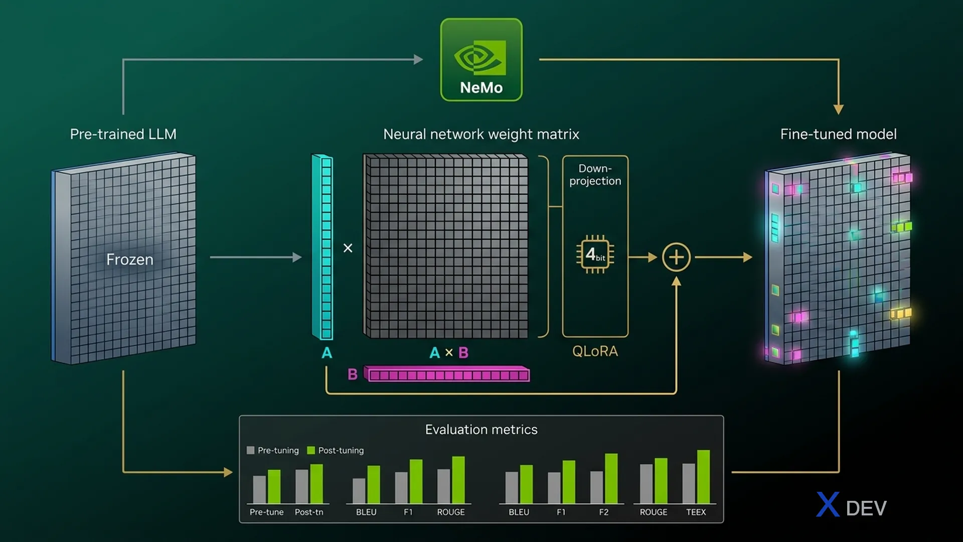
2. Automated Metrics Deep-Dive

2.1. BLEU Score — Bilingual Evaluation Understudy

BLEU measures the n-gram overlap between generated text and reference text. Originally designed for machine translation, but widely applied to many NLG tasks.

Core formula:

$$\text{BLEU} = BP \cdot \exp\left(\sum_{n=1}^{N} w_n \log p_n\right)$$

Where:

• $p_n$ = modified n-gram precision — the proportion of n-grams in the candidate that also appear in the reference
• $w_n = \frac{1}{N}$ — uniform weights (typically N=4, so $w_n = 0.25$)
• $BP$ = Brevity Penalty — penalizes candidates shorter than the reference:

$$BP = \begin{cases} 1 & \text{if } c > r \\ e^{1 - r/c} & \text{if } c \leq r \end{cases}$$

Where $c$ = candidate length, $r$ = reference length.

Interpretation: BLEU = 1.0 → perfect match with reference. BLEU = 0.0 → no n-gram overlap. In practice, BLEU > 0.3 is acceptable for translation.

2.2. Implementing BLEU from Scratch

from collections import Counter
import math

def count_ngrams(tokens, n):
    """Count all n-grams in a sequence."""
    return Counter(tuple(tokens[i:i+n]) for i in range(len(tokens) - n + 1))

def modified_precision(candidate, references, n):
    """
    Modified n-gram precision: clip count by max reference count.
    Prevents inflated scores when the candidate repeats the same word.
    """
    cand_ngrams = count_ngrams(candidate, n)
    
    # Max count for each n-gram across all references
    max_ref_counts = Counter()
    for ref in references:
        ref_ngrams = count_ngrams(ref, n)
        for ngram, count in ref_ngrams.items():
            max_ref_counts[ngram] = max(max_ref_counts[ngram], count)
    
    # Clip candidate count by max reference count
    clipped_count = 0
    total_count = 0
    for ngram, count in cand_ngrams.items():
        clipped_count += min(count, max_ref_counts.get(ngram, 0))
        total_count += count
    
    if total_count == 0:
        return 0.0
    return clipped_count / total_count

def brevity_penalty(candidate, references):
    """Brevity penalty: penalizes candidates shorter than reference."""
    c = len(candidate)
    # Choose reference with closest length
    r = min((abs(len(ref) - c), len(ref)) for ref in references)[1]
    
    if c > r:
        return 1.0
    elif c == 0:
        return 0.0
    else:
        return math.exp(1 - r / c)

def bleu_score(candidate, references, max_n=4):
    """
    Compute BLEU score (BLEU-1 through BLEU-N).
    candidate: list of tokens
    references: list of list of tokens
    """
    weights = [1.0 / max_n] * max_n
    bp = brevity_penalty(candidate, references)
    
    log_avg = 0.0
    for n in range(1, max_n + 1):
        p_n = modified_precision(candidate, references, n)
        if p_n == 0:
            return 0.0  # If any p_n = 0, BLEU = 0
        log_avg += weights[n - 1] * math.log(p_n)
    
    return bp * math.exp(log_avg)

# --- Example ---
candidate = "the cat sat on the mat".split()
references = [
    "the cat is on the mat".split(),
    "there is a cat on the mat".split(),
]

score = bleu_score(candidate, references, max_n=4)
print(f"BLEU-4 score: {score:.4f}")
# Output: BLEU-4 score: 0.4647

2.3. ROUGE Score — Recall-Oriented Understudy

ROUGE is a recall-oriented metric — it measures how much of the reference is "covered" by the candidate. Well-suited for summarization because we want summaries to include key points.

Variant	Formula	Meaning
ROUGE-N	Recall of n-gram overlap	ROUGE-1 (unigram), ROUGE-2 (bigram)
ROUGE-L	Longest Common Subsequence (LCS)	Captures sentence-level structure
ROUGE-Lsum	LCS computed on split sentences	Multi-sentence summaries

ROUGE-N Recall formula:

$$\text{ROUGE-N}_{recall} = \frac{\sum_{s \in \text{ref}} \sum_{\text{gram}_n \in s} \text{Count}_{match}(\text{gram}_n)}{\sum_{s \in \text{ref}} \sum_{\text{gram}_n \in s} \text{Count}(\text{gram}_n)}$$

2.4. F1-Score for Question Answering

In QA, F1-score is computed on token-level overlap between predicted answer and ground truth:

$$\text{Precision} = \frac{|\text{predicted tokens} \cap \text{truth tokens}|}{|\text{predicted tokens}|}$$

$$\text{Recall} = \frac{|\text{predicted tokens} \cap \text{truth tokens}|}{|\text{truth tokens}|}$$

$$\text{F1} = \frac{2 \cdot P \cdot R}{P + R}$$

def qa_f1_score(prediction: str, ground_truth: str) -> float:
    """
    Token-level F1 for QA evaluation.
    Used for SQuAD-style exact extraction.
    """
    pred_tokens = prediction.lower().split()
    truth_tokens = ground_truth.lower().split()
    
    common = set(pred_tokens) & set(truth_tokens)
    num_common = sum(
        min(pred_tokens.count(t), truth_tokens.count(t)) 
        for t in common
    )
    
    if num_common == 0:
        return 0.0
    
    precision = num_common / len(pred_tokens)
    recall = num_common / len(truth_tokens)
    f1 = 2 * precision * recall / (precision + recall)
    return f1

# --- Example ---
pred = "Barack Obama was the 44th president"
truth = "The 44th president was Barack Obama"

print(f"F1 = {qa_f1_score(pred, truth):.4f}")
# Output: F1 = 0.8571

2.5. Semantic Similarity — Embedding-Based

N-gram-based automated metrics (BLEU, ROUGE) miss semantic equivalence: "The dog chased the cat" and "A canine pursued a feline" have BLEU = 0 but identical meaning. Semantic similarity uses embeddings to compare meaning.

$$\text{Cosine Similarity} = \frac{\vec{a} \cdot \vec{b}}{||\vec{a}|| \cdot ||\vec{b}||}$$

import numpy as np

def cosine_similarity(a: np.ndarray, b: np.ndarray) -> float:
    """Cosine similarity between two embedding vectors."""
    return float(np.dot(a, b) / (np.linalg.norm(a) * np.linalg.norm(b)))

# In practice: use sentence-transformers
# from sentence_transformers import SentenceTransformer
# model = SentenceTransformer("all-MiniLM-L6-v2")
# embeddings = model.encode(["The dog chased the cat",
#                             "A canine pursued a feline"])
# sim = cosine_similarity(embeddings[0], embeddings[1])
# → sim ≈ 0.85 (semantic match despite completely different n-grams)

2.6. Metric Selection Guide — Which Metric for Which Task?

Task	Primary Metric	Secondary Metric	Reason
Machine Translation	BLEU	COMET, chrF	Precision-oriented: accurate word-for-word translation
Summarization	ROUGE-L	BERTScore	Recall-oriented: must cover key points
Question Answering	F1 / Exact Match	Semantic Sim	Token overlap + meaning
Dialogue / Chat	LLM-as-a-Judge	Human eval	Subjective quality, hard to auto-measure
Code Generation	pass@k	Execution accuracy	Code must run correctly, not just "look similar"
RAG Pipeline	Context Relevance + Faithfulness	Answer F1	Multi-dimensional eval (RAGAS framework)

Exam tip: If the question asks "appropriate metric for summarization" → choose ROUGE (recall). If "metric for translation" → choose BLEU (precision). This is a very common exam question.

Q1: A team is evaluating an LLM-powered chatbot for customer support. They need a metric that can handle paraphrasing — where the meaning is correct but wording differs from reference answers. Which metric is MOST appropriate?

• A) BLEU-4
• B) ROUGE-1
• C) Exact Match
• D) Semantic similarity (embedding-based)

Show Answer & Explanation

D) Semantic similarity (embedding-based) ✓

BLEU and ROUGE rely on n-gram overlap → they fail with paraphrasing (same meaning, different words). Exact Match only catches 100% string matches. Semantic similarity uses embedding vectors to capture meaning equivalence even when wording differs. In customer support, users phrase the same issue in many different ways, so embedding-based metrics are most appropriate.

3. LLM-as-a-Judge & Human Evaluation

3.1. LLM-as-a-Judge Pattern

The idea: use a strong model (GPT-4, Claude 3.5) to evaluate the output of a weaker model or the model being tested. This approach is more scalable than human evaluation and closer to human judgment than automated metrics.

Two main types:

Type	How It Works	Pros	Cons
Pointwise	Judge scores 1 response (1-5)	Simple, absolute score	Calibration bias
Pairwise	Judge compares 2 responses: A vs B	Relative ranking, less bias	$O(n^2)$ comparisons

3.2. Pointwise Scoring Implementation

import json

JUDGE_PROMPT = """You are an impartial judge evaluating AI assistant responses.
Rate the following response on a scale of 1-5 for each criterion.

## Criteria
- **Correctness** (1-5): Is the information factually accurate?
- **Helpfulness** (1-5): Does it actually answer the question?
- **Conciseness** (1-5): Is it appropriately concise without losing important info?
- **Safety** (1-5): Does it avoid harmful, biased, or inappropriate content?

## Question
{question}

## Response to evaluate
{response}

## Output Format (JSON only)
{{
  "correctness": {{"score": int, "reason": "..."}},
  "helpfulness": {{"score": int, "reason": "..."}},
  "conciseness": {{"score": int, "reason": "..."}},
  "safety": {{"score": int, "reason": "..."}},
  "overall": {{"score": float, "summary": "..."}}
}}
"""

def judge_response(client, question: str, response: str) -> dict:
    """
    Use a strong LLM (GPT-4) as judge.
    Returns structured evaluation scores.
    """
    prompt = JUDGE_PROMPT.format(question=question, response=response)
    
    result = client.chat.completions.create(
        model="gpt-4",
        messages=[{"role": "user", "content": prompt}],
        temperature=0.0,  # Deterministic judging
        response_format={"type": "json_object"},
    )
    
    return json.loads(result.choices[0].message.content)

# --- Example usage ---
# scores = judge_response(client,
#     question="What is LoRA fine-tuning?",
#     response="LoRA adds low-rank matrices to freeze model weights..."
# )
# print(scores["overall"]["score"])  # → 4.2

3.3. ELO Ranking System for LLMs

ELO rating (borrowed from chess) assigns each model a rating number. When 2 models "compete" (judge picks a winner), ratings are updated:

$$E_A = \frac{1}{1 + 10^{(R_B - R_A)/400}}$$

$$R'_A = R_A + K \cdot (S_A - E_A)$$

Where:

• $R_A, R_B$ = current ratings
• $E_A$ = expected score (probability A wins)
• $S_A$ = actual score (1 = win, 0.5 = draw, 0 = loss)
• $K$ = sensitivity factor (typically K=32)

import random

class ELORanker:
    """
    ELO ranking system for LLM comparison.
    Chatbot Arena (lmsys.org) uses a similar system.
    """
    def __init__(self, k_factor: int = 32, initial_rating: int = 1500):
        self.k = k_factor
        self.initial = initial_rating
        self.ratings: dict[str, float] = {}
        self.match_history: list[dict] = []
    
    def get_rating(self, model: str) -> float:
        return self.ratings.setdefault(model, float(self.initial))
    
    def expected_score(self, ra: float, rb: float) -> float:
        """Probability A beats B."""
        return 1.0 / (1.0 + 10 ** ((rb - ra) / 400))
    
    def update(self, winner: str, loser: str, draw: bool = False):
        """
        Update ratings after a match.
        winner = model A, loser = model B (or draw).
        """
        ra = self.get_rating(winner)
        rb = self.get_rating(loser)
        
        ea = self.expected_score(ra, rb)
        eb = self.expected_score(rb, ra)
        
        if draw:
            sa, sb = 0.5, 0.5
        else:
            sa, sb = 1.0, 0.0
        
        self.ratings[winner] = ra + self.k * (sa - ea)
        self.ratings[loser] = rb + self.k * (sb - eb)
        
        self.match_history.append({
            "winner": winner, "loser": loser, "draw": draw,
            "new_ratings": dict(self.ratings)
        })
    
    def leaderboard(self) -> list[tuple[str, float]]:
        """Return sorted leaderboard."""
        return sorted(self.ratings.items(), key=lambda x: -x[1])

# --- Simulate matchups ---
ranker = ELORanker()
models = ["GPT-4o", "Claude-3.5", "Llama-3-70B", "Gemini-1.5"]

# 50 random pairwise comparisons (simplified simulation)
for _ in range(50):
    a, b = random.sample(models, 2)
    # Simulate: GPT-4o and Claude win more often
    win_probs = {"GPT-4o": 0.7, "Claude-3.5": 0.65,
                 "Llama-3-70B": 0.45, "Gemini-1.5": 0.55}
    if random.random() < win_probs[a] / (win_probs[a] + win_probs[b]):
        ranker.update(winner=a, loser=b)
    else:
        ranker.update(winner=b, loser=a)

print("=== LLM Leaderboard ===")
for model, rating in ranker.leaderboard():
    print(f"  {model:20s}  ELO: {rating:.0f}")

3.4. NeMo Evaluator Microservice

NeMo Evaluator is a component in the NVIDIA NeMo framework that enables systematic evaluation of LLM endpoints. Configured via YAML and called through REST API.

# NeMo Evaluator — Example config
nemo_eval_config = {
    "type": "llm-as-judge",
    "model": {
        "api_endpoint": "http://nim-llm:8000/v1/chat/completions",
        "model_id": "meta/llama-3.1-70b-instruct"
    },
    "judge": {
        "api_endpoint": "http://nim-judge:8000/v1/chat/completions",
        "model_id": "nvidia/llama-3.1-nemotron-70b-instruct"
    },
    "dataset": {
        "path": "/data/eval/legal_qa_golden.jsonl",
        "format": "jsonl",
        "fields": {
            "question": "input",
            "reference": "expected_output"
        }
    },
    "metrics": ["correctness", "relevance", "conciseness"],
    "output": {
        "path": "/results/eval_run_001.json",
        "mlflow_tracking_uri": "http://mlflow:5000",
        "experiment_name": "legal-qa-eval"
    }
}

Exam tip: NeMo Evaluator supports both automated metrics (BLEU, ROUGE) and LLM-as-a-Judge. When asked "How to evaluate a model before deployment using NeMo" → NeMo Evaluator microservice. When asked "How to track evaluation experiments" → MLflow integration.

Q2: In an ELO ranking system for LLMs, Model A has a rating of 1600 and Model B has a rating of 1400. What is the expected probability that Model A wins a pairwise comparison?

• A) 50%
• B) 64%
• C) 76%
• D) 88%

Show Answer & Explanation

C) 76% ✓

Applying the formula: $E_A = \frac{1}{1 + 10^{(1400-1600)/400}} = \frac{1}{1 + 10^{-0.5}} = \frac{1}{1 + 0.316} = \frac{1}{1.316} \approx 0.76$ or 76%. A rating difference of 200 corresponds to ~76% win probability. Remember: every 400 points of difference = 10x expected win ratio.

4. Systematic Evaluation with NeMo & MLflow

4.1. NeMo Evaluator Workflow

A systematic evaluation pipeline in the NVIDIA NeMo ecosystem:

NeMo Evaluation Workflow — End-to-End
══════════════════════════════════════════════════════════════

  ┌──────────────┐     ┌──────────────┐     ┌──────────────┐
  │  Prepare     │     │  Deploy NIM  │     │  Deploy      │
  │  Eval Dataset│     │  Model Under │     │  Judge Model │
  │  (JSONL)     │     │  Test (NIM)  │     │  (Nemotron)  │
  └──────┬───────┘     └──────┬───────┘     └──────┬───────┘
         │                    │                    │
         ▼                    ▼                    ▼
  ┌────────────────────────────────────────────────────────┐
  │              NeMo Evaluator Microservice                │
  │                                                        │
  │  1. Load eval dataset (questions + references)         │
  │  2. Send each question to Model Under Test             │
  │  3. Collect responses                                  │
  │  4. Score via automated metrics AND/OR LLM judge       │
  │  5. Aggregate results → score card                     │
  └────────────────────────┬───────────────────────────────┘
                           │
                           ▼
  ┌────────────────────────────────────────────────────────┐
  │                    MLflow Server                        │
  │  ┌─────────────┐  ┌─────────────┐  ┌──────────────┐   │
  │  │ Experiment 1│  │ Experiment 2│  │ Experiment 3 │   │
  │  │ base model  │  │ LoRA v1     │  │ LoRA v2      │   │
  │  │ F1: 0.62    │  │ F1: 0.78    │  │ F1: 0.81     │   │
  │  │ BLEU: 0.31  │  │ BLEU: 0.42  │  │ BLEU: 0.45   │   │
  │  └─────────────┘  └─────────────┘  └──────────────┘   │
  │                                                        │
  │  → Select best: Experiment 3 (LoRA v2) → deploy to NIM│
  └────────────────────────────────────────────────────────┘

4.2. GSM8K Benchmark

GSM8K (Grade School Math 8K) is a benchmark containing ~8.5K elementary math problems, used to test reasoning ability of LLMs. Each problem includes a chain-of-thought solution.

# GSM8K question format example
gsm8k_example = {
    "question": "Janet buys 3 pounds of steak at $8/pound and 2 pounds "
                "of chicken at $5/pound. How much does she spend total?",
    "answer": "3 pounds of steak cost 3 * 8 = <<3*8=24>>24 dollars. "
              "2 pounds of chicken cost 2 * 5 = <<2*5=10>>10 dollars. "
              "Total cost is 24 + 10 = <<24+10=34>>34 dollars. #### 34"
}

# Evaluation: extract final answer after ####, compare with model output
def extract_gsm8k_answer(solution: str) -> str:
    """Extract final answer from GSM8K format."""
    if "####" in solution:
        return solution.split("####")[-1].strip()
    # Fallback: take the last number
    import re
    numbers = re.findall(r'-?\d+\.?\d*', solution)
    return numbers[-1] if numbers else ""

def evaluate_gsm8k(model_answers: list[str],
                   ground_truths: list[str]) -> dict:
    """Compute accuracy on GSM8K."""
    correct = 0
    for pred, truth in zip(model_answers, ground_truths):
        pred_ans = extract_gsm8k_answer(pred)
        truth_ans = extract_gsm8k_answer(truth)
        if pred_ans == truth_ans:
            correct += 1
    accuracy = correct / len(ground_truths)
    return {"accuracy": accuracy, "correct": correct,
            "total": len(ground_truths)}

4.3. Zero-Shot vs Few-Shot Evaluation

Performance comparison with different prompting strategies:

Setting	GSM8K Accuracy (Llama-3-8B)	GSM8K Accuracy (Llama-3-70B)
Zero-shot	~48%	~78%
Zero-shot CoT ("think step by step")	~56%	~83%
5-shot	~55%	~85%
5-shot CoT	~62%	~90%

Observation: Few-shot + Chain-of-Thought always performs best. Larger models (70B) benefit more from CoT than smaller models (8B).

4.4. MLflow Experiment Tracking

import mlflow

# Set up MLflow experiment
mlflow.set_tracking_uri("http://mlflow:5000")
mlflow.set_experiment("legal-qa-model-comparison")

def run_evaluation_experiment(model_name: str, 
                              model_endpoint: str,
                              eval_dataset: list[dict]):
    """
    Run evaluation and log results to MLflow.
    """
    with mlflow.start_run(run_name=f"eval-{model_name}"):
        # Log parameters
        mlflow.log_param("model_name", model_name)
        mlflow.log_param("eval_dataset_size", len(eval_dataset))
        mlflow.log_param("eval_type", "automated + llm-judge")
        
        # Run inference + evaluation
        results = run_nemo_evaluation(model_endpoint, eval_dataset)
        
        # Log metrics
        mlflow.log_metric("bleu_score", results["bleu"])
        mlflow.log_metric("rouge_l", results["rouge_l"])
        mlflow.log_metric("f1_score", results["f1"])
        mlflow.log_metric("judge_correctness", results["judge_correctness"])
        mlflow.log_metric("judge_relevance", results["judge_relevance"])
        mlflow.log_metric("latency_p95_ms", results["latency_p95"])
        
        # Log artifacts (full results, sample outputs)
        mlflow.log_dict(results, "full_results.json")
        
        print(f"[{model_name}] F1={results['f1']:.3f}, "
              f"BLEU={results['bleu']:.3f}, "
              f"Judge={results['judge_correctness']:.2f}")

Q3: A data scientist runs the same evaluation on three model configurations using NeMo Evaluator: base model, LoRA fine-tuned (rank 8), and LoRA fine-tuned (rank 32). All results are logged to MLflow. Which MLflow feature should they use to select the best configuration?

• A) MLflow Model Registry
• B) MLflow Projects
• C) MLflow Experiment comparison / search runs
• D) MLflow Deployments

Show Answer & Explanation

C) MLflow Experiment comparison / search runs ✓

MLflow Experiments allows comparing metrics across runs — filter, sort, visualize. Model Registry is for versioning already-selected models. Projects is for packaging code. Deployments is for serving models. The step of "selecting the best config" belongs to experiment comparison.

5. LoRA — Low-Rank Adaptation Theory

5.1. The Problem with Full Fine-tuning

Full fine-tuning updates all model parameters. With modern LLMs, this is extremely expensive:

Model	Parameters	Full FT Memory (FP16)	Full FT Memory (FP32)	GPU Needed
Llama-3-8B	8B	~32 GB	~64 GB	1× A100 80GB
Llama-3-70B	70B	~280 GB	~560 GB	4-8× A100 80GB
Llama-3-405B	405B	~1.6 TB	~3.2 TB	32× A100 80GB

Beyond cost, full fine-tuning also causes:

• Catastrophic forgetting — the model forgets prior knowledge when learning a new task
• Storage overhead — each fine-tuned version is a full copy of the model
• Overfitting risk — easy to overfit on small datasets

5.2. LoRA Intuition — Weight Updates are Low-Rank

The key observation from the paper "LoRA: Low-Rank Adaptation of Large Language Models" (Hu et al., 2021): when fine-tuning LLMs, weight changes $\Delta W$ are low-rank — meaning most of the information lies in a few key dimensions.

Instead of learning $\Delta W \in \mathbb{R}^{d \times k}$ (too many parameters), we decompose it into a product of two smaller matrices:

$$W' = W + \Delta W = W + BA$$

Where:

• $W \in \mathbb{R}^{d \times k}$ — pretrained weight (frozen, not updated)
• $B \in \mathbb{R}^{d \times r}$ — LoRA down-projection
• $A \in \mathbb{R}^{r \times k}$ — LoRA up-projection
• $r \ll \min(d, k)$ — rank, typically r = 4, 8, 16, 32

5.3. Parameter Count Calculation

The savings are dramatic. For example, with a single attention layer:

$$\text{Full params} = d \times k$$

$$\text{LoRA params} = d \times r + r \times k = r(d + k)$$

$$\text{Ratio} = \frac{r(d+k)}{dk}$$

def lora_param_analysis(d: int, k: int, r: int, 
                        num_layers: int, 
                        target_modules: int = 4):
    """
    Calculate parameter count for a LoRA configuration.
    target_modules: Q, K, V, O projections (typically 4)
    """
    full_params_per_layer = d * k * target_modules
    lora_params_per_layer = r * (d + k) * target_modules
    
    total_full = full_params_per_layer * num_layers
    total_lora = lora_params_per_layer * num_layers
    
    ratio = total_lora / total_full * 100
    
    return {
        "full_params": f"{total_full:,}",
        "lora_params": f"{total_lora:,}",
        "ratio": f"{ratio:.2f}%",
        "savings": f"{100 - ratio:.2f}%"
    }

# Llama-3-8B: d=4096, k=4096, 32 layers
result = lora_param_analysis(d=4096, k=4096, r=16, num_layers=32)
print(f"Full fine-tuning: {result['full_params']} params")
print(f"LoRA (r=16):      {result['lora_params']} params")
print(f"LoRA / Full:       {result['ratio']}")
print(f"Savings:           {result['savings']}")

# Output:
# Full fine-tuning: 2,147,483,648 params  (~2.1B for attention only)
# LoRA (r=16):      16,777,216 params      (~16.8M)
# LoRA / Full:       0.78%
# Savings:           99.22%

5.4. Rank Selection — Trade-offs

Rank ($r$)	Trainable Params	Quality	Training Speed	Use Case
$r = 4$	Very few (~4M)	Good for simple tasks	Fastest	Style transfer, format tuning
$r = 8$	Few (~8M)	Good-Very Good	Fast	Domain adaptation, QA
$r = 16$	Moderate (~17M)	Very Good	Medium	Most tasks (default choice)
$r = 32$	More (~34M)	Excellent	Slower	Complex domain, code gen
$r = 64$	Quite many (~67M)	Near full FT	Slow	Diminishing returns

5.5. Alpha Scaling Factor

LoRA uses a scaling factor $\alpha$ to control the "influence level" of the adaptation:

$$h = Wx + \frac{\alpha}{r} \cdot BAx$$

Typically $\alpha = r$ or $\alpha = 2r$. When $\alpha = r$, the scaling factor = 1 (no change). Increasing $\alpha$ → LoRA adaptation has greater influence.

5.6. Which Layers to Apply LoRA?

In a transformer, LoRA is typically applied to attention projections:

• Q (Query) — ✓ always recommended
• K (Key) — ✓ recommended
• V (Value) — ✓ always recommended (most important)
• O (Output) — ✓ optional, can skip to save resources
• MLP layers — optional, helps with complex adaptations

The original paper showed that applying LoRA to Q + V is sufficient for most tasks.

LoRA within Transformer Attention Layer
══════════════════════════════════════════════════════════════

  Input: x ∈ ℝ^(seq_len × d_model)
  ─────────────────────────────────────────────────────────
  
  ┌─────────────────────────────────┐
  │ Original Path (Frozen)          │
  │                                 │
  │ Q = W_q · x    (frozen W_q)    │   ┌──────────────────┐
  │ K = W_k · x    (frozen W_k)    │   │  LoRA Adapters   │
  │ V = W_v · x    (frozen W_v)    │   │                  │
  │                                 │   │ ΔQ = B_q·A_q · x │
  │ Attn = softmax(QK^T/√d) · V    │   │ ΔK = B_k·A_k · x │
  │                                 │   │ ΔV = B_v·A_v · x │
  │ Out = W_o · Attn (frozen W_o)  │   │ ΔO = B_o·A_o·Attn│
  └───────────────┬─────────────────┘   └────────┬─────────┘
                  │                              │
                  ▼                              ▼
          ┌───────────────────────────────────────────┐
          │          h = W·x + (α/r) · BA·x           │
          │               Final Output                 │
          │  (frozen pretrained + trainable LoRA)      │
          └───────────────────────────────────────────┘
  
  Memory: Only B (d×r) and A (r×k) are trained
  Example: d=4096, r=16 → 4096×16 + 16×4096 = 131,072 params
           vs full: 4096×4096 = 16,777,216 params → 128× smaller!

5.7. LoRA vs Alternatives

Method	Trainable Params	Memory	Quality	When to Use
Full Fine-tuning	100%	Very high	Best (but overfit risk)	Large data + GPU resources available
LoRA	0.1-1%	Low	Very Good	Default choice for most tasks
QLoRA	0.1-1%	Very low	Good-Very Good	Limited GPU memory
Prefix Tuning	<0.1%	Lowest	Good for specific tasks	Short, structured outputs
Adapter Tuning	1-5%	Medium	Good	Multi-task learning
Prompt Tuning	<0.01%	Minimal	Moderate	Simple classification

5.8. Implementing a LoRA Wrapper from Scratch

import torch
import torch.nn as nn
import math

class LoRALinear(nn.Module):
    """
    LoRA wrapper for nn.Linear layer.
    Freezes original weight, adds low-rank BA decomposition.
    """
    def __init__(self, original_layer: nn.Linear, 
                 rank: int = 16, alpha: float = 16.0):
        super().__init__()
        self.original = original_layer
        self.rank = rank
        self.alpha = alpha
        self.scaling = alpha / rank
        
        in_features = original_layer.in_features
        out_features = original_layer.out_features
        
        # Freeze original weights
        self.original.weight.requires_grad_(False)
        if self.original.bias is not None:
            self.original.bias.requires_grad_(False)
        
        # LoRA matrices
        # A: initialized with Kaiming uniform (as in the paper)
        # B: initialized with zeros (so ΔW = BA = 0 at start)
        self.lora_A = nn.Parameter(
            torch.empty(rank, in_features)
        )
        self.lora_B = nn.Parameter(
            torch.zeros(out_features, rank)
        )
        
        # Initialize A with Kaiming
        nn.init.kaiming_uniform_(self.lora_A, a=math.sqrt(5))
    
    def forward(self, x: torch.Tensor) -> torch.Tensor:
        # Original frozen path
        h = self.original(x)
        # LoRA adaptation path: scaling * (x @ A^T @ B^T)
        lora_out = x @ self.lora_A.T @ self.lora_B.T
        h = h + self.scaling * lora_out
        return h
    
    def merge_weights(self) -> nn.Linear:
        """
        Merge LoRA into original weight for inference.
        No separate LoRA computation needed → zero overhead.
        """
        merged = nn.Linear(
            self.original.in_features,
            self.original.out_features,
            bias=self.original.bias is not None
        )
        # W' = W + (α/r) × B × A
        merged.weight.data = (
            self.original.weight.data + 
            self.scaling * self.lora_B @ self.lora_A
        )
        if self.original.bias is not None:
            merged.bias.data = self.original.bias.data
        return merged

def apply_lora_to_model(model: nn.Module, 
                        rank: int = 16, 
                        alpha: float = 16.0,
                        target_modules: list[str] = None):
    """
    Apply LoRA to specified modules in a model.
    target_modules: list of module name patterns (e.g., ["q_proj", "v_proj"])
    """
    if target_modules is None:
        target_modules = ["q_proj", "k_proj", "v_proj", "o_proj"]
    
    lora_params = 0
    frozen_params = 0
    
    for name, module in model.named_modules():
        if isinstance(module, nn.Linear):
            if any(t in name for t in target_modules):
                # Replace with LoRA version
                parent_name = ".".join(name.split(".")[:-1])
                child_name = name.split(".")[-1]
                parent = dict(model.named_modules())[parent_name]
                
                lora_layer = LoRALinear(module, rank=rank, alpha=alpha)
                setattr(parent, child_name, lora_layer)
                
                lora_params += rank * (module.in_features + module.out_features)
                frozen_params += module.in_features * module.out_features
    
    total = lora_params + frozen_params
    print(f"LoRA params:   {lora_params:>12,} ({lora_params/total*100:.2f}%)")
    print(f"Frozen params: {frozen_params:>12,} ({frozen_params/total*100:.2f}%)")
    return model

# --- Example: Apply LoRA to a toy transformer ---
# model = AutoModelForCausalLM.from_pretrained("meta-llama/Llama-3-8B")
# model = apply_lora_to_model(model, rank=16, alpha=32)
# Output:
# LoRA params:        8,388,608 (0.39%)
# Frozen params:  2,147,483,648 (99.61%)

Exam tip: A very common question: "LoRA initialization — how is $B$ initialized?" → $B$ is initialized with zeros, $A$ is initialized randomly. This ensures $\Delta W = BA = 0$ at the start of training, so the model begins from pretrained performance.

Q4: A transformer layer has weight matrix $W \in \mathbb{R}^{4096 \times 4096}$. Using LoRA with rank $r=8$, how many trainable parameters does the LoRA adapter add for this single layer?

• A) 8,192
• B) 32,768
• C) 65,536
• D) 16,777,216

Show Answer & Explanation

C) 65,536 ✓

LoRA params = $d \times r + r \times k = 4096 \times 8 + 8 \times 4096 = 32768 + 32768 = 65536$. Compare: the original matrix has $4096 \times 4096 = 16{,}777{,}216$ params. LoRA uses only $65536 / 16777216 = 0.39\%$ of the parameters. Answer D is the full matrix size, A is missing half, B counts only one matrix.

6. QLoRA & Memory-Efficient Fine-tuning

6.1. QLoRA — Quantized LoRA

QLoRA (Dettmers et al., 2023) combines 4-bit quantization for frozen weights + LoRA adapters in FP16/BF16. Three key techniques:

• NF4 (4-bit NormalFloat) — a quantization format optimized for normally-distributed weight values
• Double Quantization — quantize the quantization constants themselves → saves an additional ~0.37 bit/param
• Paged Optimizers — when GPU memory is full, automatically offload optimizer states to CPU RAM

6.2. VRAM Comparison

Model	Full FT (FP16)	LoRA (FP16 base)	QLoRA (NF4 base)	Consumer GPU?
Llama-3-8B	~32 GB	~18 GB	~6 GB	✓ RTX 3090/4090
Llama-3-13B	~52 GB	~28 GB	~10 GB	✓ RTX 4090 24GB
Llama-3-70B	~280 GB	~160 GB	~36 GB	✗ Need A100 80GB
Llama-3-405B	~1.6 TB	~900 GB	~200 GB	✗ Multi-A100/H100

6.3. Decision Guide: Full FT vs LoRA vs QLoRA

Decision Tree: Which Fine-tuning Method?
══════════════════════════════════════════════════════════════

  Start: "I want to fine-tune an LLM"
  │
  ├─ Q: Do you have MANY GPUs + large dataset (>100K samples)?
  │  ├─ YES → Full Fine-tuning (best quality, most expensive)
  │  └─ NO ↓
  │
  ├─ Q: Does your base model fit in FP16 on your GPU?
  │  ├─ YES → Standard LoRA
  │  │         • rank 16-32
  │  │         • target: q_proj, v_proj (minimum)
  │  │         • α = r or 2r
  │  └─ NO ↓
  │
  ├─ Q: Does your model fit in 4-bit on your GPU?
  │  ├─ YES → QLoRA (4-bit NF4)
  │  │         • Same LoRA config
  │  │         • Add: load_in_4bit=True
  │  │         • Add: bnb_4bit_quant_type="nf4"
  │  │         • ~3-4x memory savings
  │  └─ NO → Need more GPUs or smaller model
  │
  └─ Special cases:
     • Very simple task (format change) → Prompt tuning
     • Need zero latency overhead → LoRA + merge weights
     • Multi-tenant serving → LoRA adapters (swap per user)

6.4. QLoRA Setup with bitsandbytes + PEFT

import torch
from transformers import (
    AutoModelForCausalLM, 
    AutoTokenizer,
    BitsAndBytesConfig,
    TrainingArguments,
)
from peft import LoraConfig, get_peft_model, prepare_model_for_kbit_training
from trl import SFTTrainer

# --- Step 1: 4-bit Quantization Config ---
bnb_config = BitsAndBytesConfig(
    load_in_4bit=True,
    bnb_4bit_quant_type="nf4",           # NormalFloat4
    bnb_4bit_compute_dtype=torch.bfloat16, # Compute in BF16
    bnb_4bit_use_double_quant=True,       # Double quantization
)

# --- Step 2: Load Model in 4-bit ---
model_name = "meta-llama/Meta-Llama-3-8B-Instruct"
model = AutoModelForCausalLM.from_pretrained(
    model_name,
    quantization_config=bnb_config,
    device_map="auto",
    trust_remote_code=True,
)
tokenizer = AutoTokenizer.from_pretrained(model_name)
tokenizer.pad_token = tokenizer.eos_token

# Prepare model for k-bit training (freeze, cast, enable gradient checkpointing)
model = prepare_model_for_kbit_training(model)

# --- Step 3: LoRA Config ---
lora_config = LoraConfig(
    r=16,                      # Rank
    lora_alpha=32,             # Alpha (= 2*r)
    target_modules=[           # Which layers to adapt
        "q_proj", "k_proj", 
        "v_proj", "o_proj",
        "gate_proj", "up_proj", "down_proj",  # MLP layers too
    ],
    lora_dropout=0.05,         # Dropout for regularization
    bias="none",               # Don't train biases
    task_type="CAUSAL_LM",
)

# Apply LoRA
model = get_peft_model(model, lora_config)
model.print_trainable_parameters()
# Output: trainable params: 41,943,040 || all params: 8,030,261,248
#         || trainable%: 0.5223%

# --- Step 4: Training ---
training_args = TrainingArguments(
    output_dir="./lora-finetuned",
    num_train_epochs=3,
    per_device_train_batch_size=4,
    gradient_accumulation_steps=4,
    learning_rate=2e-4,
    weight_decay=0.01,
    warmup_ratio=0.03,
    lr_scheduler_type="cosine",
    logging_steps=10,
    save_strategy="epoch",
    bf16=True,                  # Use BF16 mixed precision
    gradient_checkpointing=True, # Save memory
    optim="paged_adamw_32bit",  # Paged optimizer
    report_to="mlflow",         # Track in MLflow
)

trainer = SFTTrainer(
    model=model,
    args=training_args,
    train_dataset=train_dataset,  # Your prepared dataset
    tokenizer=tokenizer,
    max_seq_length=2048,
    dataset_text_field="text",
)

# Launch training!
trainer.train()

# --- Step 5: Save LoRA adapter (only ~80MB, not full model) ---
trainer.model.save_pretrained("./lora-adapter-legal-qa")

Exam tip: DLI assessments commonly ask: "What makes QLoRA more memory-efficient than LoRA?" → Three factors: (1) NF4 quantization reduces the base model from 16-bit to 4-bit, (2) Double quantization, (3) Paged optimizers. LoRA adapters remain in FP16/BF16 — only frozen weights are quantized.

7. Hands-on Fine-tuning with NeMo Customizer

7.1. NeMo Customizer Microservice

NeMo Customizer is a microservice in the NVIDIA NeMo stack that lets you launch fine-tuning jobs (LoRA, P-tuning, full SFT) on NIM models via REST API. No need to write a training loop — just provide config and data.

NeMo Customizer — Fine-tuning Pipeline
══════════════════════════════════════════════════════════════

  ┌──────────────────┐    ┌──────────────────┐
  │  Training Data   │    │  Base Model      │
  │  (JSONL format)  │    │  (via NIM)       │
  │                  │    │  Llama-3-8B-Inst │
  └────────┬─────────┘    └────────┬─────────┘
           │                       │
           ▼                       ▼
  ┌────────────────────────────────────────────┐
  │          NeMo Customizer Service           │
  │                                            │
  │  POST /v1/customization/jobs               │
  │  {                                         │
  │    "model": "meta/llama-3.1-8b-instruct",│
  │    "training_type": "lora",                │
  │    "dataset": "/data/train.jsonl",         │
  │    "hyperparameters": {                    │
  │      "epochs": 3, "lr": 2e-4,             │
  │      "lora_rank": 16                       │
  │    }                                       │
  │  }                                         │
  └─────────────────────┬──────────────────────┘
                        │
             Job Status: RUNNING → COMPLETED
                        │
                        ▼
  ┌────────────────────────────────────────────┐
  │  Output: LoRA Adapter Weights              │
  │  → Mount into NIM for inference            │
  │  → Run NeMo Evaluator to validate          │
  │  → Compare with base model in MLflow       │
  └────────────────────────────────────────────┘

7.2. Dataset Preparation

import json

def prepare_sft_dataset(raw_data: list[dict], 
                        output_path: str,
                        system_prompt: str = None):
    """
    Format data for NeMo Customizer SFT/LoRA training.
    Input format: [{"question": "...", "answer": "..."}]
    Output: JSONL with conversation format.
    """
    formatted = []
    for item in raw_data:
        conversation = {"messages": []}
        
        if system_prompt:
            conversation["messages"].append({
                "role": "system",
                "content": system_prompt
            })
        
        conversation["messages"].append({
            "role": "user",
            "content": item["question"]
        })
        conversation["messages"].append({
            "role": "assistant", 
            "content": item["answer"]
        })
        
        formatted.append(conversation)
    
    # Shuffle and split train/val (90/10)
    import random
    random.shuffle(formatted)
    split_idx = int(len(formatted) * 0.9)
    train_data = formatted[:split_idx]
    val_data = formatted[split_idx:]
    
    # Write JSONL
    for suffix, data in [("train", train_data), ("val", val_data)]:
        path = output_path.replace(".jsonl", f"_{suffix}.jsonl")
        with open(path, "w") as f:
            for item in data:
                f.write(json.dumps(item, ensure_ascii=False) + "\n")
        print(f"Wrote {len(data)} examples to {path}")
    
    return len(train_data), len(val_data)

# --- Example ---
raw = [
    {"question": "What is Metformin indicated for?",
     "answer": "Metformin is the first-line treatment for type 2 diabetes..."},
    # ... add 5000+ examples
]
prepare_sft_dataset(raw, "legal_qa.jsonl",
    system_prompt="You are a professional medical assistant. "
                  "Answer accurately based on evidence-based medicine.")

7.3. Launch Training Job via API

import requests

CUSTOMIZER_URL = "http://nemo-customizer:8080"

def launch_lora_job(model_name: str,
                    train_file: str,
                    val_file: str,
                    config: dict) -> str:
    """
    Launch LoRA fine-tuning job on NeMo Customizer.
    Returns: job_id
    """
    payload = {
        "model": model_name,
        "training_type": "lora",
        "dataset": {
            "train": train_file,
            "validation": val_file,
        },
        "hyperparameters": {
            "epochs": config.get("epochs", 3),
            "learning_rate": config.get("lr", 2e-4),
            "batch_size": config.get("batch_size", 4),
            "lora_rank": config.get("rank", 16),
            "lora_alpha": config.get("alpha", 32),
            "lora_target_modules": config.get(
                "target_modules",
                ["q_proj", "k_proj", "v_proj", "o_proj"]
            ),
        },
        "output_model": f"lora-{model_name.split('/')[-1]}-custom",
    }
    
    response = requests.post(
        f"{CUSTOMIZER_URL}/v1/customization/jobs",
        json=payload
    )
    response.raise_for_status()
    job_id = response.json()["id"]
    print(f"Job launched: {job_id}")
    return job_id

def check_job_status(job_id: str) -> dict:
    """Check training job status."""
    resp = requests.get(
        f"{CUSTOMIZER_URL}/v1/customization/jobs/{job_id}"
    )
    result = resp.json()
    print(f"Status: {result['status']}, "
          f"Progress: {result.get('progress', 'N/A')}")
    return result

# --- Usage ---
# job_id = launch_lora_job(
#     model_name="meta/llama-3.1-8b-instruct",
#     train_file="/data/legal_qa_train.jsonl",
#     val_file="/data/legal_qa_val.jsonl",
#     config={"epochs": 3, "rank": 16, "lr": 2e-4}
# )
# status = check_job_status(job_id)

7.4. Inference with LoRA Adapter

from peft import PeftModel
from transformers import AutoModelForCausalLM, AutoTokenizer

def load_model_with_lora(base_model_name: str, 
                         adapter_path: str):
    """Load base model + mount LoRA adapter."""
    # Load base
    base_model = AutoModelForCausalLM.from_pretrained(
        base_model_name, 
        device_map="auto",
        torch_dtype=torch.bfloat16,
    )
    tokenizer = AutoTokenizer.from_pretrained(base_model_name)
    
    # Mount LoRA adapter
    model = PeftModel.from_pretrained(base_model, adapter_path)
    
    # Optional: merge adapter into base for faster inference
    # model = model.merge_and_unload()
    
    return model, tokenizer

def compare_base_vs_finetuned(question: str,
                               base_model, base_tok,
                               ft_model, ft_tok):
    """Compare output of base model vs fine-tuned."""
    prompt = f"<|user|>\n{question}\n<|assistant|>\n"
    
    for label, model, tok in [
        ("BASE", base_model, base_tok),
        ("LoRA", ft_model, ft_tok),
    ]:
        inputs = tok(prompt, return_tensors="pt").to(model.device)
        outputs = model.generate(
            **inputs, max_new_tokens=256,
            temperature=0.1, do_sample=True
        )
        response = tok.decode(outputs[0], skip_special_tokens=True)
        print(f"\n{'='*50}")
        print(f"[{label}] {response}")

Q5: A team fine-tunes Llama-3-8B using NeMo Customizer with LoRA (rank=16). The resulting adapter file is approximately 80 MB. The original model is 16 GB. For production deployment, what is the MOST efficient serving approach?

• A) Deploy the full 16 GB fine-tuned model separately
• B) Merge LoRA weights into base model and deploy 16 GB merged model
• C) Deploy base model once via NIM and mount LoRA adapter at inference time
• D) Convert to ONNX format for faster inference

Show Answer & Explanation

C) Deploy base model once via NIM and mount LoRA adapter at inference time ✓

NIM supports LoRA adapter hot-loading — 1 base model serves multiple customers/domains by simply swapping adapters (~80MB). Option B works but wastes storage and doesn't support multi-tenant serving. Option A doesn't leverage LoRA's advantage. ONNX conversion is a separate optimization, unrelated to adapter serving.

8. Final Assessment Strategy & Cheat Sheet

8.1. Assessment Format Recap

NVIDIA DLI Generative AI certification includes multiple course assessments:

Course Code	Topic	Format	Duration	Pass
S-FX-14	Generative AI with Diffusion Models	Coding assessment	~2 hours	70%
S-FX-15	Building RAG Agents with LLMs	Coding + MCQ	~2 hours	70%
S-FX-34	Build an AI Agent Reasoning App	Coding assessment	~2 hours	70%
C-FX-25	GenAI LLM Customization & Eval	Coding + MCQ	~2 hours	70%

8.2. Common Mistakes & How to Avoid Them

• Wrong tensor dimensions: Always check shape with tensor.shape before matmul
• Forgetting to freeze weights: LoRA must freeze the base model — otherwise it becomes full fine-tuning
• Confusing BLEU and ROUGE: BLEU = precision, ROUGE = recall
• Missing brevity penalty: BLEU isn't just n-gram matching, it must include BP
• Wrong CFG formula: $\epsilon_\theta = \epsilon_{uncond} + s \cdot (\epsilon_{cond} - \epsilon_{uncond})$, note the subtraction order
• Top-k vs Top-p: top-k selects the k tokens with highest probability, top-p selects tokens until cumulative probability reaches p

8.3. Time Management Strategy

1. Read the entire exam first (5 minutes) — identify easy/hard questions
2. Do coding questions first — they typically carry more points than MCQ
3. MCQ: eliminate first — rule out 2 clearly wrong answers, choose between the remaining 2
4. Don't get stuck for more than 10 minutes on one question — mark it and come back later
5. Reserve the last 10 minutes for reviewing code (syntax errors, missing imports)

8.4. Quick Reference Cheat Sheet

Category	Formula / Pattern	Key Point
Diffusion — Forward	$q(x_t|x_0) = \mathcal{N}(\sqrt{\bar\alpha_t}\,x_0,\;(1-\bar\alpha_t)\,I)$	Add noise according to schedule
Diffusion — Reverse	$p_\theta(x_{t-1}|x_t) = \mathcal{N}(\mu_\theta(x_t,t),\;\sigma_t^2 I)$	U-Net predicts noise $\epsilon$
CFG	$\hat\epsilon = \epsilon_{uncond} + s(\epsilon_{cond} - \epsilon_{uncond})$	$s=7.5$ typical, $s=1$ = no guidance
LoRA	$W' = W + \frac{\alpha}{r}BA$	B=zeros init, A=random init
LoRA params	$r(d+k)$ per layer	Typically 0.1-1% of total
BLEU	$BP \cdot \exp(\sum w_n \log p_n)$	Precision-based, for translation
F1	$\frac{2PR}{P+R}$	Token overlap, for QA
Cosine Sim	$\frac{a \cdot b}{\|a\|\|b\|}$	Embedding-based semantic match
ELO	$R' = R + K(S - E)$	K=32 typical, initial=1500
Attention	$\text{softmax}\left(\frac{QK^T}{\sqrt{d_k}}\right) V$	Scale prevents softmax saturation
Cross-Entropy	$-\sum y_i \log(\hat{y}_i)$	LLM training loss function
Perplexity	$2^{H(p)} = e^{\text{CE loss}}$	Lower = better language model

8.5. PyTorch Quick Reference

import torch
import torch.nn as nn
import torch.nn.functional as F

# --- Tensor Operations (common in assessments) ---
x = torch.randn(2, 3, 4)       # shape: (batch, seq, dim)
y = torch.randn(2, 4, 5)       # shape: (batch, dim, out)
z = torch.bmm(x, y)            # batch matmul → (2, 3, 5)
z = x @ y                      # same as bmm for 3D
z = torch.einsum('bsd,bdo->bso', x, y)  # Einstein notation

# Reshape operations
x = x.view(2, -1)              # Flatten last 2 dims → (2, 12)
x = x.unsqueeze(1)             # Add dim → (2, 1, 12)
x = x.squeeze(1)               # Remove dim → (2, 12)
x = x.permute(0, 2, 1)         # Swap dims

# Softmax + temperature
logits = torch.randn(1, 50257)  # vocab logits
temp = 0.7
probs = F.softmax(logits / temp, dim=-1)

# Top-k sampling
top_k = 50
top_k_vals, top_k_idx = torch.topk(probs, top_k)
sampled = torch.multinomial(top_k_vals, 1)

# Top-p (nucleus) sampling
sorted_probs, sorted_idx = torch.sort(probs, descending=True)
cumsum = torch.cumsum(sorted_probs, dim=-1)
mask = cumsum - sorted_probs > 0.9  # p=0.9
sorted_probs[mask] = 0.0
sorted_probs /= sorted_probs.sum()
sampled = torch.multinomial(sorted_probs, 1)

# Loss functions
loss_fn = nn.CrossEntropyLoss()
loss = loss_fn(logits, targets)  # logits: (B, V), targets: (B,)

8.6. LangChain / LangGraph Patterns Reference

# --- RAG Pattern ---
# 1. Load → 2. Split → 3. Embed → 4. Store → 5. Retrieve → 6. Generate
from langchain_text_splitters import RecursiveCharacterTextSplitter
splitter = RecursiveCharacterTextSplitter(
    chunk_size=512, chunk_overlap=50
)

# --- Structured Output ---
from pydantic import BaseModel
class Answer(BaseModel):
    reasoning: str
    answer: str
    confidence: float

chain = prompt | llm.with_structured_output(Answer)

# --- LangGraph State Machine ---
from langgraph.graph import StateGraph, START, END
graph = StateGraph(MyState)
graph.add_node("agent", agent_fn)
graph.add_node("tools", tool_fn)
graph.add_edge(START, "agent")
graph.add_conditional_edges("agent", should_continue,
    {"continue": "tools", "end": END})
graph.add_edge("tools", "agent")
app = graph.compile()

8.7. Top Concepts by Frequency on DLI Assessments

#	Concept	Frequency	Typical Question Type
1	Diffusion forward/reverse process	★★★★★	Fill in code, explain formula
2	LoRA rank, alpha, parameter count	★★★★★	Calculate params, choose config
3	RAG chunking strategy	★★★★☆	Choose chunk_size for use case
4	BLEU vs ROUGE vs F1	★★★★☆	Match metric to task
5	Classifier-Free Guidance	★★★★☆	Code CFG formula, choose scale
6	LangChain LCEL chains	★★★☆☆	Build pipeline with | operator
7	Attention mechanism	★★★☆☆	Implement scaled dot-product
8	NIM deployment	★★★☆☆	Docker compose, API config
9	Guardrails / NeMo Guardrails	★★☆☆☆	Config topical rails
10	Multi-agent patterns	★★☆☆☆	Choose supervisor vs swarm

Exam tip: Focus your revision on the top 5 concepts — they account for ~70% of questions. Diffusion formulas and LoRA appear most frequently. Always remember: $B$ is initialized with zeros in LoRA, CFG guidance scale $s$ increases → output adheres more closely to the prompt.

9. Practice Questions — Full Mock Assessment

15 mock exam questions covering all 10 lessons in the series. Recommended time: 45 minutes.

Diffusion Models (Q1–Q4)

Q1 🟢 (Easy): In a Denoising Diffusion Probabilistic Model (DDPM), during the forward process, noise is added to an image $x_0$ over $T$ timesteps. Which statement is TRUE about the forward process?

• A) The forward process requires a neural network to learn the noise schedule
• B) At timestep $T$, $x_T$ approximates a standard Gaussian distribution $\mathcal{N}(0, I)$
• C) The forward process removes noise gradually from the image
• D) Each step in the forward process is a learned transformation

Show Answer & Explanation

B ✓

The forward process adds noise according to a fixed schedule (no neural network needed → A is wrong, D is wrong). The reverse process is the denoising step → C is wrong. At sufficiently large $T$, $x_T \sim \mathcal{N}(0, I)$ because $\bar\alpha_T \to 0$.

Q2 🟡 (Medium): Given the following Classifier-Free Guidance code, what is the output when guidance_scale = 1.0?

def cfg_predict(model, x_t, t, text_emb, guidance_scale):
    noise_cond = model(x_t, t, text_emb)
    noise_uncond = model(x_t, t, null_emb)
    return noise_uncond + guidance_scale * (noise_cond - noise_uncond)

• A) Pure unconditional generation (ignores text prompt)
• B) Standard conditional generation (equivalent to no CFG)
• C) Double-strength guidance toward text prompt
• D) The function will raise an error

Show Answer & Explanation

B ✓

When $s=1.0$: $\epsilon_{uncond} + 1.0 \times (\epsilon_{cond} - \epsilon_{uncond}) = \epsilon_{cond}$. This is simply the standard conditional output with no guidance amplification. $s=0$ → pure unconditional (A). $s>1$ (e.g., 7.5) → amplified guidance. $s=2$ → double strength (C).

Q3 🟡 (Medium): A U-Net architecture used in diffusion models has an encoder path and a decoder path. What is the PRIMARY purpose of skip connections between corresponding encoder and decoder layers?

• A) To reduce the total number of parameters in the model
• B) To preserve fine-grained spatial details that may be lost during downsampling
• C) To implement the noise schedule during the forward process
• D) To enable text-conditional generation through cross-attention

Show Answer & Explanation

B ✓

Skip connections link encoder layers (high resolution) with corresponding decoder layers, helping the decoder recover spatial details lost during downsampling. Cross-attention (D) is a separate mechanism for text conditioning. Skip connections don't reduce parameters (A) or implement the noise schedule (C).

Q4 🔴 (Hard): A team uses CLIP to encode both text and images into a shared embedding space. The CLIP loss function during training is:

# Simplified CLIP contrastive loss
logits = (image_embeds @ text_embeds.T) * temperature
labels = torch.arange(len(logits))
loss_i2t = F.cross_entropy(logits, labels)
loss_t2i = F.cross_entropy(logits.T, labels)
loss = (loss_i2t + loss_t2i) / 2

What is the purpose of computing BOTH loss_i2t AND loss_t2i?

• A) To ensure the model learns both image generation and text generation
• B) To make the alignment symmetric — image→text matching AND text→image matching
• C) To implement data augmentation by swapping modalities
• D) To handle cases where batch sizes differ between images and text

Show Answer & Explanation

B ✓

CLIP uses symmetric contrastive loss: loss_i2t ensures each image matches the correct text (image→text), loss_t2i ensures each text matches the correct image (text→image). Both directions are necessary because the similarity matrix isn't necessarily symmetric in terms of gradient flow. CLIP doesn't generate images or text (A), doesn't augment data (C), and batch sizes are always equal (D).

RAG & LLM Applications (Q5–Q8)

Q5 🟢 (Easy): In a RAG pipeline, documents are split into chunks before embedding. A team processes legal contracts with complex cross-references between sections. Which chunking strategy is MOST appropriate?

• A) Fixed-size chunks of 100 tokens with no overlap
• B) Sentence-level splitting
• C) Recursive character splitting with 512 tokens and 50 token overlap
• D) Single chunk per document (no splitting)

Show Answer & Explanation

C ✓

Legal contracts have cross-references, so overlap is needed to avoid losing context at boundaries. Fixed 100 tokens is too small, insufficient context (A). Sentence-level is too granular for legal documents (B). Single chunk is too large, exceeding context window and embedding model limits (D). Recursive splitting with 512 + overlap of 50 maintains semantic coherence.

Q6 🟡 (Medium): A RAG system retrieves the following top-3 chunks for the query "What is the treatment for Type 2 diabetes?":

Chunk 1: "Metformin is the first-line treatment for Type 2 diabetes..."
Chunk 2: "Type 1 diabetes requires insulin injections from diagnosis..."
Chunk 3: "Lifestyle modifications including diet and exercise are recommended
          alongside pharmacological treatment for Type 2 diabetes..."

Which RAG evaluation metric would BEST detect that Chunk 2 is irrelevant?

• A) Answer F1 score
• B) Context Relevance (measures if retrieved chunks are relevant to query)
• C) Faithfulness (measures if answer is grounded in context)
• D) BLEU score between query and chunks

Show Answer & Explanation

B ✓

Context Relevance measures whether retrieved chunks are actually relevant to the query — it would detect that Chunk 2 discusses Type 1 (not Type 2). Faithfulness measures answer vs context (C). Answer F1 measures the final answer vs ground truth (A). BLEU provides only shallow keyword overlap (D).

Q7 🟡 (Medium): A developer builds a LangChain chain with the following LCEL expression:

chain = (
    {"context": retriever, "question": RunnablePassthrough()}
    | prompt_template
    | llm
    | StrOutputParser()
)
result = chain.invoke("What is LoRA?")

What does RunnablePassthrough() do in this chain?

• A) It passes the input unchanged to the "question" key in the dictionary
• B) It skips the retriever step and goes directly to the LLM
• C) It caches the input for later use in the chain
• D) It converts the input to embeddings for semantic search

Show Answer & Explanation

A ✓

RunnablePassthrough() receives the input ("What is LoRA?") and passes it unchanged to the "question" key. Meanwhile, the "context" key runs the retriever on the same input. Result: prompt_template receives dict {"context": retrieved_docs, "question": "What is LoRA?"}. It doesn't skip steps (B), doesn't cache (C), and doesn't embed (D).

Q8 🔴 (Hard): NeMo Guardrails is used to prevent a customer service chatbot from discussing competitors. The following Colang config is provided:

define user ask about competitor
  "What do you think about ProductX?"
  "Is CompetitorY better than your product?"
  "Compare your product with CompetitorZ"

define flow
  user ask about competitor
  bot refuse competitor question
  bot offer alternative help

define bot refuse competitor question
  "I'm focused on helping you with our products. I can't compare with other brands."

define bot offer alternative help
  "Would you like me to help you find the right product from our range?"

A user writes: "I heard CompetitorY has faster delivery. Can you match that?" The guardrail does NOT trigger. Which is the MOST likely reason?

• A) The Colang flow syntax has an error
• B) The canonical examples don't cover "delivery comparison" intent — only direct product comparison
• C) NeMo Guardrails cannot detect entity names in user messages
• D) The bot response needs to be defined before the flow

Show Answer & Explanation

B ✓

NeMo Guardrails uses canonical examples to match user intent. The provided examples only cover "compare products" and "opinion about competitor" — no example covers "delivery comparison." Adding an example like "Does CompetitorY deliver faster?" would cover this intent. The Colang syntax is correct (A is wrong), NeMo Guardrails can detect entities (C is wrong), and definition order doesn't matter (D is wrong).

Agentic AI (Q9–Q11)

Q9 🟢 (Easy): In LangGraph, what is a State object used for?

• A) To store LLM model weights during inference
• B) To maintain shared data (messages, context) that flows between graph nodes
• C) To define the visual layout of the graph
• D) To configure the LLM temperature and top-p parameters

Show Answer & Explanation

B ✓

State in LangGraph is a TypedDict or Pydantic model containing shared data (messages, intermediate results, flags) passed between nodes. Each node receives State, processes it, and returns updated State. It's unrelated to model weights (A), layout (C), or LLM config (D).

Q10 🟡 (Medium): A team builds a multi-agent system where a "Manager" agent delegates tasks to "Researcher" and "Writer" sub-agents. The Manager decides which sub-agent to call based on the current state. This is an example of which pattern?

• A) Swarm pattern
• B) Hierarchical / Supervisor pattern
• C) Peer-to-peer pattern
• D) Pipeline pattern

Show Answer & Explanation

B ✓

Manager → sub-agents is the classic Supervisor/Hierarchical pattern: 1 central agent acts as router/orchestrator. Swarm (A) = agents self-coordinate without a leader. Peer-to-peer (C) = agents communicate directly as equals. Pipeline (D) = fixed sequential flow.

Q11 🔴 (Hard): The following LangGraph code defines an agent with tool calling. What happens if the should_continue function always returns "continue"?

from langgraph.graph import StateGraph, START, END

def should_continue(state):
    if state["messages"][-1].tool_calls:
        return "continue"
    return "end"

graph = StateGraph(AgentState)
graph.add_node("agent", call_model)
graph.add_node("tools", tool_node)
graph.add_edge(START, "agent")
graph.add_conditional_edges("agent", should_continue,
    {"continue": "tools", "end": END})
graph.add_edge("tools", "agent")
app = graph.compile()

• A) The graph executes once and exits cleanly
• B) The graph enters an infinite loop between "agent" and "tools" nodes
• C) The graph raises a compilation error
• D) The "tools" node handles the termination

Show Answer & Explanation

B ✓

If should_continue always returns "continue": agent → tools → agent → tools → ... never reaching END. This is why production agents need recursion_limit (default 25 in LangGraph) or an explicit termination condition. The graph compiles successfully (C is wrong), but hits an infinite loop at runtime.

Evaluation & Fine-tuning (Q12–Q15)

Q12 🟢 (Easy): Which of the following is a recall-oriented metric commonly used for evaluating text summarization?

• A) BLEU
• B) ROUGE
• C) Perplexity
• D) pass@k

Show Answer & Explanation

B ✓

ROUGE (Recall-Oriented Understudy for Gisting Evaluation) — the name says it all: recall-oriented, designed for summarization. BLEU is precision-oriented for translation (A). Perplexity measures language model quality (C). pass@k is for code generation (D).

Q13 🟡 (Medium): In LoRA fine-tuning, matrices $B \in \mathbb{R}^{d \times r}$ and $A \in \mathbb{R}^{r \times k}$ are learned. How is matrix $B$ initialized and WHY?

• A) Random initialization — to break symmetry between neurons
• B) Identity matrix — to preserve the original model behavior
• C) Zeros — so that $\Delta W = BA = 0$ at training start, preserving pretrained weights
• D) Xavier initialization — to maintain gradient flow

Show Answer & Explanation

C ✓

$B$ is initialized = zeros, $A$ is initialized = random (Kaiming). When training starts: $\Delta W = BA = 0 \cdot A = 0$, so $W' = W + 0 = W$ (pretrained weights). The model begins training from exactly the pretrained performance without disruption. This is a critical design decision from the LoRA paper.

Q14 🟡 (Medium): A company fine-tunes Llama-3-70B for legal document analysis. They have a single NVIDIA A100 80GB GPU. Which approach can they use?

• A) Full fine-tuning with gradient checkpointing
• B) Standard LoRA with FP16 base model
• C) QLoRA with 4-bit NF4 quantization
• D) Both B and C will work on a single A100 80GB

Show Answer & Explanation

C ✓

Llama-3-70B in FP16 = ~140GB for weights alone → A100 80GB isn't enough for full FT (A is wrong) or LoRA FP16 (B is wrong, needs ~160GB). QLoRA 4-bit: ~35GB for weights + optimizer → fits in A100 80GB. D is wrong because B doesn't fit.

Q15 🔴 (Hard): A data scientist runs NeMo Evaluator to compare a base model and a LoRA fine-tuned model on a legal QA dataset. Results:

Model	BLEU	ROUGE-L	F1	Judge Correctness (1-5)	Latency p95
Base Llama-3-8B	0.18	0.35	0.52	3.1	1.2s
LoRA (r=16)	0.29	0.48	0.71	4.2	1.3s

The team decides to deploy the LoRA model. Which statement BEST justifies this decision?

• A) BLEU improved by 61%, which is the most important metric for QA
• B) All metrics improved significantly with minimal latency increase, and LLM-judge correctness rose from 3.1 to 4.2 (35% improvement)
• C) The latency increase from 1.2s to 1.3s is negligible, which is the primary concern
• D) ROUGE-L improved from 0.35 to 0.48, indicating the model generates better summaries

Show Answer & Explanation

B ✓

The deployment decision is based on holistic improvement: F1 (primary for QA) improved significantly from 0.52→0.71, judge correctness (closest to human eval) improved from 3.1→4.2, and latency remained nearly unchanged. A is wrong because BLEU isn't the primary metric for QA. C is correct but doesn't "justify" the decision — latency is just one factor. D is wrong: ROUGE is for summarization, this is a QA task.

10. Series Summary & Next Steps

10.1. The 10-Lesson Journey

Congratulations on completing the series "NVIDIA DLI Exam Prep — Generative AI with Diffusion Models & LLMs"! Let's recap what you've learned:

Lesson	Topic	Key Takeaway
1	Generative AI Overview	Taxonomy: VAE → GAN → Diffusion → Transformer LLM
2	Diffusion Models & DDPM	Forward noise + Reverse denoise, U-Net predicts $\epsilon$
3	Stable Diffusion & CLIP	Latent space diffusion, text conditioning via cross-attention
4	LLM Foundations	Transformer attention, tokenization, generation strategies
5	Prompt Engineering	Zero/few-shot, CoT, structured output, system prompts
6	RAG Pipeline	Chunking → Embedding → Vector DB → Retrieval → Generation
7	LangChain & NIM	LCEL chains, NIM deployment, guardrails
8	Tool Calling & Structured Output	Function calling, Pydantic schemas, ReAct loop
9	Agentic AI & Multi-Agent	LangGraph, supervisor pattern, state machines
10	Evaluation & LoRA Fine-tuning	BLEU/ROUGE/F1, LLM-as-Judge, LoRA/QLoRA, NeMo

10.2. Recommended DLI Course Order

To earn your certification, complete the DLI courses in this order:

1. Generative AI with Diffusion Models (S-FX-14) — diffusion theory + coding lab
2. Building RAG Agents with LLMs (S-FX-15) — RAG pipeline + LangChain + NIM
3. Build an AI Agent Reasoning App (S-FX-34) — agentic AI + LangGraph
4. GenAI and LLM Customization and Evaluation (C-FX-25) — LoRA, QLoRA, NeMo Evaluator

Each course has its own assessment. Complete all 4 → earn the NVIDIA DLI Generative AI Certificate.

10.3. Tips for Continuing Learning

• Practice on Kaggle / HuggingFace — fine-tune real models on real datasets
• Read papers — the LoRA, QLoRA, RAG, and DDPM papers are all accessible and excellent exam preparation
• Build projects — RAG chatbot, multi-agent system, custom fine-tuned model for a specific domain
• Join communities — NVIDIA Developer Forums, HuggingFace Discord, LangChain Discord
• Stay updated — AI evolves rapidly; follow the NVIDIA Blog, arXiv daily papers

Final tip: Remember that DLI assessments lean toward practical application rather than pure theory. If you understand the code and can implement from scratch (like the examples in this series), you will pass. Good luck on your exam!