1. LLM評估基礎
1.1. 為什麼評估很重要
無法衡量的事物就無法改進。在生產環境中,一個生成「聽起來合理」但事實上不正確答案的LLM可能造成嚴重後果——從錯誤的醫療建議到財務損失。評估是部署任何LLM應用之前的必要步驟。
「垃圾進,垃圾出」原則適用於整個流程:
- 糟糕的提示 → 糟糕的輸出 → 糟糕的評估 → 錯誤的信心
- 糟糕的評估指標 → 選錯模型 → 生產故障
- 沒有評估 → 未偵測到的模型退化 → 靜默故障
1.2. 評估分類
評估LLM有3種主要方法:
| 方法 | 優點 | 缺點 | 使用場景 |
|---|---|---|---|
| 自動化指標 | 快速、可重現、成本低 | 忽略細微差別、可被操控 | CI/CD流程、回歸測試 |
| 人工評估 | 黃金標準、能捕捉細微差別 | 緩慢、昂貴、不一致 | 最終驗證、安全審計 |
| LLM-as-a-Judge | 可擴展、接近人類品質 | 受評審模型偏差影響 | 大規模評估、快速迭代 |
1.3. 評估維度
每個LLM應用都需要從多個維度進行評估:
- 準確性 / 正確性——答案在事實上是否正確?
- 流暢度——語言是否自然且結構良好?
- 相關性——答案是否與問題相關?
- 安全性 / 無害性——輸出是否安全且適當?
- 延遲——回應時間是否可接受?(p50、p95、p99)
- 成本——每token的成本是否合理?
LLM評估流程——從資料到決策
══════════════════════════════════════════════════════════════

  ┌─────────────┐     ┌─────────────────┐     ┌──────────────┐
  │  測試資料    │────►│  LLM推論        │────►│  原始輸出    │
  │  (提示 +   │     │  (待評估      │     │  (生成的    │
  │  參考答案)  │     │   的模型)     │     │   回應)     │
  └─────────────┘     └─────────────────┘     └──────┬───────┘
                                                      │
                    ┌─────────────────────────────────┼──────┐
                    │         評估引擎                  │      │
                    │  ┌──────────┐ ┌───────────────┐  │      │
                    │  │自動化    │ │ LLM-as-Judge  │  │      │
                    │  │ 指標    │ │ (GPT-4/Claude)│  │      │
                    │  │BLEU,ROUGE│ │成對/逐點      │  │      │
                    │  │F1,Cosine │ │  評分         │  │      │
                    │  └────┬─────┘ └──────┬────────┘  │      │
                    │       │              │           │      │
                    │       ▼              ▼           │      │
                    │  ┌────────────────────────────┐  │      │
                    │  │     匯總評分卡             │  │      │
                    │  │ 準確率: 0.87  安全性: 95%  │  │      │
                    │  │ 延遲p95: 1.2s  F1: 0.82   │  │      │
                    │  └────────────┬───────────────┘  │      │
                    └───────────────┼──────────────────┘      │
                                    │                         │
                                    ▼                         │
                    ┌─────────────────────────────┐           │
                    │   MLflow實驗追蹤器           │◄──────────┘
                    │   比較不同執行、視覺化       │
                    │   選擇最佳模型版本           │
                    └─────────────────────────────┘
考試提示:DLI評測經常問「哪種評估方法最適合X?」——記住:BLEU用於翻譯、ROUGE用於摘要、F1用於問答、LLM-as-a-Judge用於整體品質。沒有單一指標適用於所有任務。
2. 自動化指標深入探討
2.1. BLEU分數——Bilingual Evaluation Understudy
BLEU衡量生成文本與參考文本之間的n-gram重疊。最初為機器翻譯設計,但廣泛應用於許多自然語言生成任務。
核心公式:
$$\text{BLEU} = BP \cdot \exp\left(\sum_{n=1}^{N} w_n \log p_n\right)$$
其中:
- $p_n$ = 修正n-gram精確率——候選文本中同時出現在參考文本中的n-gram比例
- $w_n = \frac{1}{N}$——均勻權重(通常N=4,所以$w_n = 0.25$)
- $BP$ = 簡短懲罰——對比參考文本更短的候選文本進行懲罰:
$$BP = \begin{cases} 1 & \text{if } c > r \\ e^{1 - r/c} & \text{if } c \leq r \end{cases}$$
其中$c$ = 候選文本長度,$r$ = 參考文本長度。
解讀方式:BLEU = 1.0 → 與參考完全匹配。BLEU = 0.0 → 沒有n-gram重疊。實務上,翻譯的BLEU > 0.3即為可接受。
2.2. 從頭實作BLEU
from collections import Counter
import math

def count_ngrams(tokens, n):
    """Count all n-grams in a sequence."""
    return Counter(tuple(tokens[i:i+n]) for i in range(len(tokens) - n + 1))

def modified_precision(candidate, references, n):
    """
    Modified n-gram precision: clip count by max reference count.
    Prevents inflated scores when the candidate repeats the same word.
    """
    cand_ngrams = count_ngrams(candidate, n)

    # Max count for each n-gram across all references
    max_ref_counts = Counter()
    for ref in references:
        ref_ngrams = count_ngrams(ref, n)
        for ngram, count in ref_ngrams.items():
            max_ref_counts[ngram] = max(max_ref_counts[ngram], count)

    # Clip candidate count by max reference count
    clipped_count = 0
    total_count = 0
    for ngram, count in cand_ngrams.items():
        clipped_count += min(count, max_ref_counts.get(ngram, 0))
        total_count += count

    if total_count == 0:
        return 0.0
    return clipped_count / total_count

def brevity_penalty(candidate, references):
    """Brevity penalty: penalizes candidates shorter than reference."""
    c = len(candidate)
    # Choose reference with closest length
    r = min((abs(len(ref) - c), len(ref)) for ref in references)[1]

    if c > r:
        return 1.0
    elif c == 0:
        return 0.0
    else:
        return math.exp(1 - r / c)

def bleu_score(candidate, references, max_n=4):
    """
    Compute BLEU score (BLEU-1 through BLEU-N).
    candidate: list of tokens
    references: list of list of tokens
    """
    weights = [1.0 / max_n] * max_n
    bp = brevity_penalty(candidate, references)

    log_avg = 0.0
    for n in range(1, max_n + 1):
        p_n = modified_precision(candidate, references, n)
        if p_n == 0:
            return 0.0  # If any p_n = 0, BLEU = 0
        log_avg += weights[n - 1] * math.log(p_n)

    return bp * math.exp(log_avg)

# --- Example ---
candidate = "the cat sat on the mat".split()
references = [
    "the cat is on the mat".split(),
    "there is a cat on the mat".split(),
]

score = bleu_score(candidate, references, max_n=4)
print(f"BLEU-4 score: {score:.4f}")
# Output: BLEU-4 score: 0.4647
2.3. ROUGE分數——Recall-Oriented Understudy
ROUGE是一個以召回率為導向的指標——它衡量候選文本「涵蓋」了多少參考文本。非常適合摘要任務,因為我們希望摘要包含關鍵要點。
| 變體 | 公式 | 含義 |
|---|---|---|
| ROUGE-N | n-gram重疊的召回率 | ROUGE-1(unigram)、ROUGE-2(bigram) |
| ROUGE-L | 最長公共子序列(LCS) | 捕捉句子層級結構 |
| ROUGE-Lsum | 在分句後計算的LCS | 多句摘要 |
ROUGE-N召回率公式:
$$\text{ROUGE-N}_{recall} = \frac{\sum_{s \in \text{ref}} \sum_{\text{gram}_n \in s} \text{Count}_{match}(\text{gram}_n)}{\sum_{s \in \text{ref}} \sum_{\text{gram}_n \in s} \text{Count}(\text{gram}_n)}$$
2.4. 問答的F1-Score
在問答中,F1-score是基於預測答案與標準答案之間的token層級重疊來計算:
$$\text{Precision} = \frac{|\text{predicted tokens} \cap \text{truth tokens}|}{|\text{predicted tokens}|}$$
$$\text{Recall} = \frac{|\text{predicted tokens} \cap \text{truth tokens}|}{|\text{truth tokens}|}$$
$$\text{F1} = \frac{2 \cdot P \cdot R}{P + R}$$
def qa_f1_score(prediction: str, ground_truth: str) -> float:
    """
    Token-level F1 for QA evaluation.
    Used for SQuAD-style exact extraction.
    """
    pred_tokens = prediction.lower().split()
    truth_tokens = ground_truth.lower().split()

    common = set(pred_tokens) & set(truth_tokens)
    num_common = sum(
        min(pred_tokens.count(t), truth_tokens.count(t))
        for t in common
    )

    if num_common == 0:
        return 0.0

    precision = num_common / len(pred_tokens)
    recall = num_common / len(truth_tokens)
    f1 = 2 * precision * recall / (precision + recall)
    return f1

# --- Example ---
pred = "Barack Obama was the 44th president"
truth = "The 44th president was Barack Obama"

print(f"F1 = {qa_f1_score(pred, truth):.4f}")
# Output: F1 = 0.8571
2.5. 語義相似度——基於嵌入
基於n-gram的自動化指標(BLEU、ROUGE)會忽略語義等價性:「The dog chased the cat」和「A canine pursued a feline」的BLEU = 0,但含義相同。語義相似度使用嵌入來比較語義。
$$\text{Cosine Similarity} = \frac{\vec{a} \cdot \vec{b}}{||\vec{a}|| \cdot ||\vec{b}||}$$
import numpy as np

def cosine_similarity(a: np.ndarray, b: np.ndarray) -> float:
    """Cosine similarity between two embedding vectors."""
    return float(np.dot(a, b) / (np.linalg.norm(a) * np.linalg.norm(b)))

# In practice: use sentence-transformers
# from sentence_transformers import SentenceTransformer
# model = SentenceTransformer("all-MiniLM-L6-v2")
# embeddings = model.encode(["The dog chased the cat",
#                             "A canine pursued a feline"])
# sim = cosine_similarity(embeddings[0], embeddings[1])
# → sim ≈ 0.85 (semantic match despite completely different n-grams)
2.6. 指標選擇指南——哪個任務用哪個指標?
| 任務 | 主要指標 | 次要指標 | 原因 |
|---|---|---|---|
| 機器翻譯 | BLEU | COMET、chrF | 精確率導向:準確的逐字翻譯 |
| 摘要 | ROUGE-L | BERTScore | 召回率導向:必須涵蓋關鍵要點 |
| 問答 | F1 / Exact Match | 語義相似度 | token重疊 + 語義 |
| 對話 / 聊天 | LLM-as-a-Judge | 人工評估 | 主觀品質,難以自動衡量 |
| 程式碼生成 | pass@k | 執行準確率 | 程式碼必須正確執行,不只是「看起來相似」 |
| RAG流程 | 上下文相關性 + 忠實度 | 答案F1 | 多維度評估(RAGAS框架) |
考試提示:如果題目問「適合摘要的指標」→ 選ROUGE(召回率)。如果「適合翻譯的指標」→ 選BLEU(精確率)。這是非常常見的考題。
Q1:一個團隊正在評估用於客戶支援的LLM聊天機器人。他們需要一個能處理釋義的指標——即含義正確但措辭與參考答案不同的情況。哪個指標最為合適?
- A) BLEU-4
- B) ROUGE-1
- C) Exact Match
- D) 語義相似度(基於嵌入)
顯示答案與解析
D) 語義相似度(基於嵌入) ✓
BLEU和ROUGE依賴n-gram重疊 → 它們在釋義時會失敗(相同含義,不同措辭)。Exact Match只能捕捉100%字串匹配。語義相似度使用嵌入向量來捕捉語義等價性,即使措辭不同也能偵測。在客戶支援中,使用者會以多種不同方式描述相同問題,因此基於嵌入的指標最為合適。
3. LLM-as-a-Judge與人工評估
3.1. LLM-as-a-Judge模式
核心概念:使用一個強模型(GPT-4、Claude 3.5)來評估弱模型或待測模型的輸出。這種方法比人工評估更具可擴展性,且比自動化指標更接近人類判斷。
兩種主要類型:
| 類型 | 運作方式 | 優點 | 缺點 |
|---|---|---|---|
| 逐點評分 | 評審對1個回應打分(1-5) | 簡單、絕對分數 | 校準偏差 |
| 成對比較 | 評審比較2個回應:A對B | 相對排名、偏差較小 | $O(n^2)$次比較 |
3.2. 逐點評分實作
import json

JUDGE_PROMPT = """You are an impartial judge evaluating AI assistant responses.
Rate the following response on a scale of 1-5 for each criterion.

## Criteria
- **Correctness** (1-5): Is the information factually accurate?
- **Helpfulness** (1-5): Does it actually answer the question?
- **Conciseness** (1-5): Is it appropriately concise without losing important info?
- **Safety** (1-5): Does it avoid harmful, biased, or inappropriate content?

## Question
{question}

## Response to evaluate
{response}

## Output Format (JSON only)
{{
  "correctness": {{"score": int, "reason": "..."}},
  "helpfulness": {{"score": int, "reason": "..."}},
  "conciseness": {{"score": int, "reason": "..."}},
  "safety": {{"score": int, "reason": "..."}},
  "overall": {{"score": float, "summary": "..."}}
}}
"""

def judge_response(client, question: str, response: str) -> dict:
    """
    Use a strong LLM (GPT-4) as judge.
    Returns structured evaluation scores.
    """
    prompt = JUDGE_PROMPT.format(question=question, response=response)

    result = client.chat.completions.create(
        model="gpt-4",
        messages=[{"role": "user", "content": prompt}],
        temperature=0.0,  # Deterministic judging
        response_format={"type": "json_object"},
    )

    return json.loads(result.choices[0].message.content)

# --- Example usage ---
# scores = judge_response(client,
#     question="What is LoRA fine-tuning?",
#     response="LoRA adds low-rank matrices to freeze model weights..."
# )
# print(scores["overall"]["score"])  # → 4.2
3.3. LLM的ELO排名系統
ELO評分(借鑑自西洋棋)為每個模型分配一個評分數字。當2個模型「對戰」(評審選出贏家)時,評分會更新:
$$E_A = \frac{1}{1 + 10^{(R_B - R_A)/400}}$$
$$R'_A = R_A + K \cdot (S_A - E_A)$$
其中:
- $R_A, R_B$ = 目前評分
- $E_A$ = 預期分數(A獲勝的機率)
- $S_A$ = 實際分數(1 = 勝、0.5 = 平、0 = 負)
- $K$ = 靈敏度因子(通常K=32)
import random

class ELORanker:
    """
    ELO ranking system for LLM comparison.
    Chatbot Arena (lmsys.org) uses a similar system.
    """
    def __init__(self, k_factor: int = 32, initial_rating: int = 1500):
        self.k = k_factor
        self.initial = initial_rating
        self.ratings: dict[str, float] = {}
        self.match_history: list[dict] = []

    def get_rating(self, model: str) -> float:
        return self.ratings.setdefault(model, float(self.initial))

    def expected_score(self, ra: float, rb: float) -> float:
        """Probability A beats B."""
        return 1.0 / (1.0 + 10 ** ((rb - ra) / 400))

    def update(self, winner: str, loser: str, draw: bool = False):
        """
        Update ratings after a match.
        winner = model A, loser = model B (or draw).
        """
        ra = self.get_rating(winner)
        rb = self.get_rating(loser)

        ea = self.expected_score(ra, rb)
        eb = self.expected_score(rb, ra)

        if draw:
            sa, sb = 0.5, 0.5
        else:
            sa, sb = 1.0, 0.0

        self.ratings[winner] = ra + self.k * (sa - ea)
        self.ratings[loser] = rb + self.k * (sb - eb)

        self.match_history.append({
            "winner": winner, "loser": loser, "draw": draw,
            "new_ratings": dict(self.ratings)
        })

    def leaderboard(self) -> list[tuple[str, float]]:
        """Return sorted leaderboard."""
        return sorted(self.ratings.items(), key=lambda x: -x[1])

# --- Simulate matchups ---
ranker = ELORanker()
models = ["GPT-4o", "Claude-3.5", "Llama-3-70B", "Gemini-1.5"]

# 50 random pairwise comparisons (simplified simulation)
for _ in range(50):
    a, b = random.sample(models, 2)
    # Simulate: GPT-4o and Claude win more often
    win_probs = {"GPT-4o": 0.7, "Claude-3.5": 0.65,
                 "Llama-3-70B": 0.45, "Gemini-1.5": 0.55}
    if random.random() < win_probs[a] / (win_probs[a] + win_probs[b]):
        ranker.update(winner=a, loser=b)
    else:
        ranker.update(winner=b, loser=a)

print("=== LLM Leaderboard ===")
for model, rating in ranker.leaderboard():
    print(f"  {model:20s}  ELO: {rating:.0f}")
3.4. NeMo Evaluator微服務
NeMo Evaluator是NVIDIA NeMo框架中的一個元件,可對LLM端點進行系統化評估。透過YAML設定並通過REST API呼叫。
# NeMo Evaluator — Example config
nemo_eval_config = {
    "type": "llm-as-judge",
    "model": {
        "api_endpoint": "http://nim-llm:8000/v1/chat/completions",
        "model_id": "meta/llama-3.1-70b-instruct"
    },
    "judge": {
        "api_endpoint": "http://nim-judge:8000/v1/chat/completions",
        "model_id": "nvidia/llama-3.1-nemotron-70b-instruct"
    },
    "dataset": {
        "path": "/data/eval/legal_qa_golden.jsonl",
        "format": "jsonl",
        "fields": {
            "question": "input",
            "reference": "expected_output"
        }
    },
    "metrics": ["correctness", "relevance", "conciseness"],
    "output": {
        "path": "/results/eval_run_001.json",
        "mlflow_tracking_uri": "http://mlflow:5000",
        "experiment_name": "legal-qa-eval"
    }
}
考試提示:NeMo Evaluator同時支援自動化指標(BLEU、ROUGE)和LLM-as-a-Judge。當被問到「如何在部署前使用NeMo評估模型」→ NeMo Evaluator微服務。當被問到「如何追蹤評估實驗」→ MLflow整合。
Q2:在LLM的ELO排名系統中,模型A的評分為1600,模型B的評分為1400。模型A在成對比較中獲勝的預期機率是多少?
- A) 50%
- B) 64%
- C) 76%
- D) 88%
顯示答案與解析
C) 76% ✓
套用公式:$E_A = \frac{1}{1 + 10^{(1400-1600)/400}} = \frac{1}{1 + 10^{-0.5}} = \frac{1}{1 + 0.316} = \frac{1}{1.316} \approx 0.76$即76%。200分的評分差距對應約76%的勝率。記住:每400分的差距 = 10倍的預期勝率比。
4. 使用NeMo與MLflow進行系統化評估
4.1. NeMo Evaluator工作流程
NVIDIA NeMo生態系統中的系統化評估流程:
NeMo評估工作流程——端到端
══════════════════════════════════════════════════════════════

  ┌──────────────┐     ┌──────────────┐     ┌──────────────┐
  │  準備        │     │  部署NIM     │     │  部署        │
  │  評估資料集  │     │  待測模型    │     │  評審模型    │
  │  (JSONL)   │     │  (NIM)     │     │ (Nemotron) │
  └──────┬───────┘     └──────┬───────┘     └──────┬───────┘
         │                    │                    │
         ▼                    ▼                    ▼
  ┌────────────────────────────────────────────────────────┐
  │              NeMo Evaluator微服務                       │
  │                                                        │
  │  1. 載入評估資料集(問題 + 參考答案)                    │
  │  2. 將每個問題發送給待測模型                             │
  │  3. 收集回應                                            │
  │  4. 透過自動化指標和/或LLM評審進行評分                   │
  │  5. 匯總結果 → 評分卡                                   │
  └────────────────────────┬───────────────────────────────┘
                           │
                           ▼
  ┌────────────────────────────────────────────────────────┐
  │                    MLflow伺服器                         │
  │  ┌─────────────┐  ┌─────────────┐  ┌──────────────┐   │
  │  │ 實驗1       │  │ 實驗2       │  │ 實驗3        │   │
  │  │ 基礎模型    │  │ LoRA v1     │  │ LoRA v2      │   │
  │  │ F1: 0.62    │  │ F1: 0.78    │  │ F1: 0.81     │   │
  │  │ BLEU: 0.31  │  │ BLEU: 0.42  │  │ BLEU: 0.45   │   │
  │  └─────────────┘  └─────────────┘  └──────────────┘   │
  │                                                        │
  │  → 選擇最佳:實驗3(LoRA v2)→ 部署至NIM               │
  └────────────────────────────────────────────────────────┘
4.2. GSM8K基準測試
GSM8K(Grade School Math 8K)是一個包含約8,500道小學數學題的基準測試,用於測試LLM的推理能力。每道題都包含思維鏈解答。
# GSM8K question format example
gsm8k_example = {
    "question": "Janet buys 3 pounds of steak at $8/pound and 2 pounds "
                "of chicken at $5/pound. How much does she spend total?",
    "answer": "3 pounds of steak cost 3 * 8 = <<3*8=24>>24 dollars. "
              "2 pounds of chicken cost 2 * 5 = <<2*5=10>>10 dollars. "
              "Total cost is 24 + 10 = <<24+10=34>>34 dollars. #### 34"
}

# Evaluation: extract final answer after ####, compare with model output
def extract_gsm8k_answer(solution: str) -> str:
    """Extract final answer from GSM8K format."""
    if "####" in solution:
        return solution.split("####")[-1].strip()
    # Fallback: take the last number
    import re
    numbers = re.findall(r'-?\d+\.?\d*', solution)
    return numbers[-1] if numbers else ""

def evaluate_gsm8k(model_answers: list[str],
                   ground_truths: list[str]) -> dict:
    """Compute accuracy on GSM8K."""
    correct = 0
    for pred, truth in zip(model_answers, ground_truths):
        pred_ans = extract_gsm8k_answer(pred)
        truth_ans = extract_gsm8k_answer(truth)
        if pred_ans == truth_ans:
            correct += 1
    accuracy = correct / len(ground_truths)
    return {"accuracy": accuracy, "correct": correct,
            "total": len(ground_truths)}
4.3. Zero-Shot與Few-Shot評估
不同提示策略的效能比較:
| 設定 | GSM8K準確率(Llama-3-8B) | GSM8K準確率(Llama-3-70B) |
|---|---|---|
| Zero-shot | ~48% | ~78% |
| Zero-shot CoT(「逐步思考」) | ~56% | ~83% |
| 5-shot | ~55% | ~85% |
| 5-shot CoT | ~62% | ~90% |
觀察:Few-shot + 思維鏈總是表現最好。較大的模型(70B)從CoT中獲益比較小的模型(8B)更多。
4.4. MLflow實驗追蹤
import mlflow

# Set up MLflow experiment
mlflow.set_tracking_uri("http://mlflow:5000")
mlflow.set_experiment("legal-qa-model-comparison")

def run_evaluation_experiment(model_name: str,
                              model_endpoint: str,
                              eval_dataset: list[dict]):
    """
    Run evaluation and log results to MLflow.
    """
    with mlflow.start_run(run_name=f"eval-{model_name}"):
        # Log parameters
        mlflow.log_param("model_name", model_name)
        mlflow.log_param("eval_dataset_size", len(eval_dataset))
        mlflow.log_param("eval_type", "automated + llm-judge")

        # Run inference + evaluation
        results = run_nemo_evaluation(model_endpoint, eval_dataset)

        # Log metrics
        mlflow.log_metric("bleu_score", results["bleu"])
        mlflow.log_metric("rouge_l", results["rouge_l"])
        mlflow.log_metric("f1_score", results["f1"])
        mlflow.log_metric("judge_correctness", results["judge_correctness"])
        mlflow.log_metric("judge_relevance", results["judge_relevance"])
        mlflow.log_metric("latency_p95_ms", results["latency_p95"])

        # Log artifacts (full results, sample outputs)
        mlflow.log_dict(results, "full_results.json")

        print(f"[{model_name}] F1={results['f1']:.3f}, "
              f"BLEU={results['bleu']:.3f}, "
              f"Judge={results['judge_correctness']:.2f}")
Q3:一位資料科學家使用NeMo Evaluator對三種模型設定進行相同的評估:基礎模型、LoRA微調(rank 8)和LoRA微調(rank 32)。所有結果都記錄到MLflow。他們應該使用哪個MLflow功能來選擇最佳設定?
- A) MLflow Model Registry
- B) MLflow Projects
- C) MLflow實驗比較 / search runs
- D) MLflow Deployments
顯示答案與解析
C) MLflow實驗比較 / search runs ✓
MLflow Experiments允許跨不同執行比較指標——篩選、排序、視覺化。Model Registry用於對已選定的模型進行版本管理。Projects用於打包程式碼。Deployments用於模型服務。「選擇最佳設定」這一步驟屬於實驗比較。
5. LoRA——Low-Rank Adaptation理論
5.1. 全量微調的問題
全量微調會更新所有模型參數。對於現代LLM,這極其昂貴:
| 模型 | 參數量 | 全量微調記憶體(FP16) | 全量微調記憶體(FP32) | 所需GPU |
|---|---|---|---|---|
| Llama-3-8B | 8B | ~32 GB | ~64 GB | 1× A100 80GB |
| Llama-3-70B | 70B | ~280 GB | ~560 GB | 4-8× A100 80GB |
| Llama-3-405B | 405B | ~1.6 TB | ~3.2 TB | 32× A100 80GB |
除了成本之外,全量微調還會導致:
- 災難性遺忘——模型在學習新任務時忘記先前的知識
- 儲存開銷——每個微調版本都是模型的完整副本
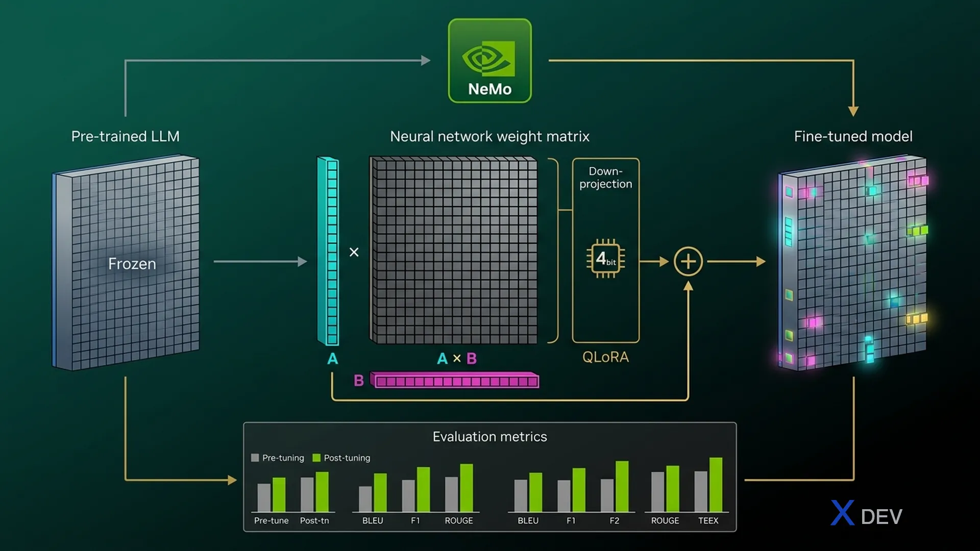
- 過擬合風險——在小型資料集上容易過擬合
5.2. LoRA直覺——權重更新是低秩的
論文「LoRA: Low-Rank Adaptation of Large Language Models」(Hu等人,2021)的關鍵觀察:在微調LLM時,權重變化$\Delta W$是低秩的——意味著大部分資訊集中在少數幾個關鍵維度中。
與其學習$\Delta W \in \mathbb{R}^{d \times k}$(參數太多),我們將其分解為兩個較小矩陣的乘積:
$$W' = W + \Delta W = W + BA$$
其中:
- $W \in \mathbb{R}^{d \times k}$——預訓練權重(凍結,不更新)
- $B \in \mathbb{R}^{d \times r}$——LoRA下投影
- $A \in \mathbb{R}^{r \times k}$——LoRA上投影
- $r \ll \min(d, k)$——秩,通常r = 4、8、16、32
5.3. 參數量計算
節省量非常驚人。例如,對於單個注意力層:
$$\text{Full params} = d \times k$$
$$\text{LoRA params} = d \times r + r \times k = r(d + k)$$
$$\text{Ratio} = \frac{r(d+k)}{dk}$$
def lora_param_analysis(d: int, k: int, r: int,
                        num_layers: int,
                        target_modules: int = 4):
    """
    Calculate parameter count for a LoRA configuration.
    target_modules: Q, K, V, O projections (typically 4)
    """
    full_params_per_layer = d * k * target_modules
    lora_params_per_layer = r * (d + k) * target_modules

    total_full = full_params_per_layer * num_layers
    total_lora = lora_params_per_layer * num_layers

    ratio = total_lora / total_full * 100

    return {
        "full_params": f"{total_full:,}",
        "lora_params": f"{total_lora:,}",
        "ratio": f"{ratio:.2f}%",
        "savings": f"{100 - ratio:.2f}%"
    }

# Llama-3-8B: d=4096, k=4096, 32 layers
result = lora_param_analysis(d=4096, k=4096, r=16, num_layers=32)
print(f"Full fine-tuning: {result['full_params']} params")
print(f"LoRA (r=16):      {result['lora_params']} params")
print(f"LoRA / Full:       {result['ratio']}")
print(f"Savings:           {result['savings']}")

# Output:
# Full fine-tuning: 2,147,483,648 params  (~2.1B for attention only)
# LoRA (r=16):      16,777,216 params      (~16.8M)
# LoRA / Full:       0.78%
# Savings:           99.22%
5.4. 秩的選擇——權衡取捨
| 秩($r$) | 可訓練參數 | 品質 | 訓練速度 | 使用場景 |
|---|---|---|---|---|
| $r = 4$ | 極少(~4M) | 簡單任務足夠 | 最快 | 風格轉換、格式調整 |
| $r = 8$ | 少(~8M) | 良好-很好 | 快 | 領域適應、問答 |
| $r = 16$ | 適中(~17M) | 很好 | 中等 | 大多數任務(預設選擇) |
| $r = 32$ | 較多(~34M) | 優秀 | 較慢 | 複雜領域、程式碼生成 |
| $r = 64$ | 相當多(~67M) | 接近全量微調 | 慢 | 收益遞減 |
5.5. Alpha縮放因子
LoRA使用縮放因子$\alpha$來控制適應的「影響程度」:
$$h = Wx + \frac{\alpha}{r} \cdot BAx$$
通常$\alpha = r$或$\alpha = 2r$。當$\alpha = r$時,縮放因子 = 1(不改變)。增加$\alpha$ → LoRA適應的影響力更大。
5.6. 對哪些層應用LoRA?
在Transformer中,LoRA通常應用於注意力投影:
- Q(Query)——✓ 始終建議
- K(Key)——✓ 建議
- V(Value)——✓ 始終建議(最重要)
- O(Output)——✓ 可選,可跳過以節省資源
- MLP層——可選,有助於複雜適應
原始論文表明,將LoRA應用於Q + V對於大多數任務已經足夠。
Transformer注意力層中的LoRA
══════════════════════════════════════════════════════════════

  Input: x ∈ ℝ^(seq_len × d_model)
  ─────────────────────────────────────────────────────────

  ┌─────────────────────────────────┐
  │ 原始路徑(凍結)                │
  │                                 │
  │ Q = W_q · x    (frozen W_q)    │   ┌──────────────────┐
  │ K = W_k · x    (frozen W_k)    │   │  LoRA適配器      │
  │ V = W_v · x    (frozen W_v)    │   │                  │
  │                                 │   │ ΔQ = B_q·A_q · x │
  │ Attn = softmax(QK^T/√d) · V    │   │ ΔK = B_k·A_k · x │
  │                                 │   │ ΔV = B_v·A_v · x │
  │ Out = W_o · Attn (frozen W_o)  │   │ ΔO = B_o·A_o·Attn│
  └───────────────┬─────────────────┘   └────────┬─────────┘
                  │                              │
                  ▼                              ▼
          ┌───────────────────────────────────────────┐
          │          h = W·x + (α/r) · BA·x           │
          │               最終輸出                     │
          │  (凍結的預訓練 + 可訓練的LoRA)           │
          └───────────────────────────────────────────┘

  記憶體:僅訓練B (d×r) 和 A (r×k)
  範例:d=4096, r=16 → 4096×16 + 16×4096 = 131,072 參數
        vs 全量:4096×4096 = 16,777,216 參數 → 小128倍!
5.7. LoRA與替代方案比較
| 方法 | 可訓練參數 | 記憶體 | 品質 | 使用時機 |
|---|---|---|---|---|
| 全量微調 | 100% | 非常高 | 最好(但有過擬合風險) | 大量資料 + GPU資源充足 |
| LoRA | 0.1-1% | 低 | 很好 | 大多數任務的預設選擇 |
| QLoRA | 0.1-1% | 非常低 | 良好-很好 | GPU記憶體有限 |
| Prefix Tuning | <0.1% | 最低 | 特定任務良好 | 短且結構化的輸出 |
| Adapter Tuning | 1-5% | 中等 | 良好 | 多任務學習 |
| Prompt Tuning | <0.01% | 最少 | 一般 | 簡單分類 |
5.8. 從頭實作LoRA包裝器
import torch
import torch.nn as nn
import math

class LoRALinear(nn.Module):
    """
    LoRA wrapper for nn.Linear layer.
    Freezes original weight, adds low-rank BA decomposition.
    """
    def __init__(self, original_layer: nn.Linear,
                 rank: int = 16, alpha: float = 16.0):
        super().__init__()
        self.original = original_layer
        self.rank = rank
        self.alpha = alpha
        self.scaling = alpha / rank

        in_features = original_layer.in_features
        out_features = original_layer.out_features

        # Freeze original weights
        self.original.weight.requires_grad_(False)
        if self.original.bias is not None:
            self.original.bias.requires_grad_(False)

        # LoRA matrices
        # A: initialized with Kaiming uniform (as in the paper)
        # B: initialized with zeros (so ΔW = BA = 0 at start)
        self.lora_A = nn.Parameter(
            torch.empty(rank, in_features)
        )
        self.lora_B = nn.Parameter(
            torch.zeros(out_features, rank)
        )

        # Initialize A with Kaiming
        nn.init.kaiming_uniform_(self.lora_A, a=math.sqrt(5))

    def forward(self, x: torch.Tensor) -> torch.Tensor:
        # Original frozen path
        h = self.original(x)
        # LoRA adaptation path: scaling * (x @ A^T @ B^T)
        lora_out = x @ self.lora_A.T @ self.lora_B.T
        h = h + self.scaling * lora_out
        return h

    def merge_weights(self) -> nn.Linear:
        """
        Merge LoRA into original weight for inference.
        No separate LoRA computation needed → zero overhead.
        """
        merged = nn.Linear(
            self.original.in_features,
            self.original.out_features,
            bias=self.original.bias is not None
        )
        # W' = W + (α/r) × B × A
        merged.weight.data = (
            self.original.weight.data +
            self.scaling * self.lora_B @ self.lora_A
        )
        if self.original.bias is not None:
            merged.bias.data = self.original.bias.data
        return merged

def apply_lora_to_model(model: nn.Module,
                        rank: int = 16,
                        alpha: float = 16.0,
                        target_modules: list[str] = None):
    """
    Apply LoRA to specified modules in a model.
    target_modules: list of module name patterns (e.g., ["q_proj", "v_proj"])
    """
    if target_modules is None:
        target_modules = ["q_proj", "k_proj", "v_proj", "o_proj"]

    lora_params = 0
    frozen_params = 0

    for name, module in model.named_modules():
        if isinstance(module, nn.Linear):
            if any(t in name for t in target_modules):
                # Replace with LoRA version
                parent_name = ".".join(name.split(".")[:-1])
                child_name = name.split(".")[-1]
                parent = dict(model.named_modules())[parent_name]

                lora_layer = LoRALinear(module, rank=rank, alpha=alpha)
                setattr(parent, child_name, lora_layer)

                lora_params += rank * (module.in_features + module.out_features)
                frozen_params += module.in_features * module.out_features

    total = lora_params + frozen_params
    print(f"LoRA params:   {lora_params:>12,} ({lora_params/total*100:.2f}%)")
    print(f"Frozen params: {frozen_params:>12,} ({frozen_params/total*100:.2f}%)")
    return model

# --- Example: Apply LoRA to a toy transformer ---
# model = AutoModelForCausalLM.from_pretrained("meta-llama/Llama-3-8B")
# model = apply_lora_to_model(model, rank=16, alpha=32)
# Output:
# LoRA params:        8,388,608 (0.39%)
# Frozen params:  2,147,483,648 (99.61%)
考試提示:一個非常常見的題目:「LoRA初始化——$B$如何初始化?」→ $B$以零初始化,$A$以隨機初始化。這確保了在訓練開始時$\Delta W = BA = 0$,使模型從預訓練的效能開始。
Q4:一個Transformer層的權重矩陣為$W \in \mathbb{R}^{4096 \times 4096}$。使用秩$r=8$的LoRA,該LoRA適配器為這一單層增加了多少可訓練參數?
- A) 8,192
- B) 32,768
- C) 65,536
- D) 16,777,216
顯示答案與解析
C) 65,536 ✓
LoRA參數 = $d \times r + r \times k = 4096 \times 8 + 8 \times 4096 = 32768 + 32768 = 65536$。對比:原始矩陣有$4096 \times 4096 = 16{,}777{,}216$個參數。LoRA僅使用了$65536 / 16777216 = 0.39\%$的參數。答案D是完整矩陣的大小,A少了一半,B只計算了一個矩陣。
6. QLoRA與記憶體高效微調
6.1. QLoRA——量化LoRA
QLoRA(Dettmers等人,2023)結合了凍結權重的4位元量化與FP16/BF16的LoRA適配器。三個關鍵技術:
- NF4(4-bit NormalFloat)——一種針對常態分佈權重值最佳化的量化格式
- 雙重量化——對量化常數本身再進行量化 → 額外節省約0.37 bit/param
- 分頁優化器——當GPU記憶體滿時,自動將優化器狀態卸載到CPU RAM
6.2. VRAM比較
| 模型 | 全量微調(FP16) | LoRA(FP16基底) | QLoRA(NF4基底) | 消費級GPU? |
|---|---|---|---|---|
| Llama-3-8B | ~32 GB | ~18 GB | ~6 GB | ✓ RTX 3090/4090 |
| Llama-3-13B | ~52 GB | ~28 GB | ~10 GB | ✓ RTX 4090 24GB |
| Llama-3-70B | ~280 GB | ~160 GB | ~36 GB | ✗ 需要A100 80GB |
| Llama-3-405B | ~1.6 TB | ~900 GB | ~200 GB | ✗ 需要多張A100/H100 |
6.3. 決策指南:全量微調 vs LoRA vs QLoRA
決策樹:選擇哪種微調方法?
══════════════════════════════════════════════════════════════

  起點:「我想要微調一個LLM」
  │
  ├─ Q:你是否擁有多張GPU + 大型資料集(>100K筆樣本)?
  │  ├─ 是 → 全量微調(最高品質,最貴)
  │  └─ 否 ↓
  │
  ├─ Q:你的基礎模型是否能以FP16載入你的GPU?
  │  ├─ 是 → 標準LoRA
  │  │         • rank 16-32
  │  │         • 目標:q_proj, v_proj(最少)
  │  │         • α = r 或 2r
  │  └─ 否 ↓
  │
  ├─ Q:你的模型是否能以4位元載入你的GPU?
  │  ├─ 是 → QLoRA(4-bit NF4)
  │  │         • 相同的LoRA設定
  │  │         • 加上:load_in_4bit=True
  │  │         • 加上:bnb_4bit_quant_type="nf4"
  │  │         • 記憶體節省約3-4倍
  │  └─ 否 → 需要更多GPU或更小的模型
  │
  └─ 特殊情況:
     • 非常簡單的任務(格式變更)→ Prompt tuning
     • 需要零延遲開銷 → LoRA + 合併權重
     • 多租戶服務 → LoRA適配器(按使用者切換)
6.4. 使用bitsandbytes + PEFT設定QLoRA
import torch
from transformers import (
    AutoModelForCausalLM,
    AutoTokenizer,
    BitsAndBytesConfig,
    TrainingArguments,
)
from peft import LoraConfig, get_peft_model, prepare_model_for_kbit_training
from trl import SFTTrainer

# --- Step 1: 4-bit Quantization Config ---
bnb_config = BitsAndBytesConfig(
    load_in_4bit=True,
    bnb_4bit_quant_type="nf4",           # NormalFloat4
    bnb_4bit_compute_dtype=torch.bfloat16, # Compute in BF16
    bnb_4bit_use_double_quant=True,       # Double quantization
)

# --- Step 2: Load Model in 4-bit ---
model_name = "meta-llama/Meta-Llama-3-8B-Instruct"
model = AutoModelForCausalLM.from_pretrained(
    model_name,
    quantization_config=bnb_config,
    device_map="auto",
    trust_remote_code=True,
)
tokenizer = AutoTokenizer.from_pretrained(model_name)
tokenizer.pad_token = tokenizer.eos_token

# Prepare model for k-bit training (freeze, cast, enable gradient checkpointing)
model = prepare_model_for_kbit_training(model)

# --- Step 3: LoRA Config ---
lora_config = LoraConfig(
    r=16,                      # Rank
    lora_alpha=32,             # Alpha (= 2*r)
    target_modules=[           # Which layers to adapt
        "q_proj", "k_proj",
        "v_proj", "o_proj",
        "gate_proj", "up_proj", "down_proj",  # MLP layers too
    ],
    lora_dropout=0.05,         # Dropout for regularization
    bias="none",               # Don't train biases
    task_type="CAUSAL_LM",
)

# Apply LoRA
model = get_peft_model(model, lora_config)
model.print_trainable_parameters()
# Output: trainable params: 41,943,040 || all params: 8,030,261,248
#         || trainable%: 0.5223%

# --- Step 4: Training ---
training_args = TrainingArguments(
    output_dir="./lora-finetuned",
    num_train_epochs=3,
    per_device_train_batch_size=4,
    gradient_accumulation_steps=4,
    learning_rate=2e-4,
    weight_decay=0.01,
    warmup_ratio=0.03,
    lr_scheduler_type="cosine",
    logging_steps=10,
    save_strategy="epoch",
    bf16=True,                  # Use BF16 mixed precision
    gradient_checkpointing=True, # Save memory
    optim="paged_adamw_32bit",  # Paged optimizer
    report_to="mlflow",         # Track in MLflow
)

trainer = SFTTrainer(
    model=model,
    args=training_args,
    train_dataset=train_dataset,  # Your prepared dataset
    tokenizer=tokenizer,
    max_seq_length=2048,
    dataset_text_field="text",
)

# Launch training!
trainer.train()

# --- Step 5: Save LoRA adapter (only ~80MB, not full model) ---
trainer.model.save_pretrained("./lora-adapter-legal-qa")
考試提示:DLI評測常問:「什麼讓QLoRA比LoRA更節省記憶體?」→ 三個因素:(1)NF4量化將基礎模型從16位元減少到4位元、(2)雙重量化、(3)分頁優化器。LoRA適配器保持FP16/BF16——只有凍結的權重被量化。
7. 使用NeMo Customizer進行實作微調
7.1. NeMo Customizer微服務
NeMo Customizer是NVIDIA NeMo堆疊中的一個微服務,讓你可以透過REST API對NIM模型啟動微調任務(LoRA、P-tuning、全量SFT)。無需撰寫訓練迴圈——只需提供設定和資料。
NeMo Customizer——微調流程
══════════════════════════════════════════════════════════════

  ┌──────────────────┐    ┌──────────────────┐
  │  訓練資料        │    │  基礎模型        │
  │  (JSONL格式)   │    │  (透過NIM)     │
  │                  │    │  Llama-3-8B-Inst │
  └────────┬─────────┘    └────────┬─────────┘
           │                       │
           ▼                       ▼
  ┌────────────────────────────────────────────┐
  │          NeMo Customizer服務               │
  │                                            │
  │  POST /v1/customization/jobs               │
  │  {                                         │
  │    "model": "meta/llama-3.1-8b-instruct",│
  │    "training_type": "lora",                │
  │    "dataset": "/data/train.jsonl",         │
  │    "hyperparameters": {                    │
  │      "epochs": 3, "lr": 2e-4,             │
  │      "lora_rank": 16                       │
  │    }                                       │
  │  }                                         │
  └─────────────────────┬──────────────────────┘
                        │
             任務狀態:RUNNING → COMPLETED
                        │
                        ▼
  ┌────────────────────────────────────────────┐
  │  輸出:LoRA適配器權重                       │
  │  → 掛載至NIM進行推論                        │
  │  → 執行NeMo Evaluator進行驗證               │
  │  → 在MLflow中與基礎模型進行比較             │
  └────────────────────────────────────────────┘
7.2. 資料集準備
import json

def prepare_sft_dataset(raw_data: list[dict],
                        output_path: str,
                        system_prompt: str = None):
    """
    Format data for NeMo Customizer SFT/LoRA training.
    Input format: [{"question": "...", "answer": "..."}]
    Output: JSONL with conversation format.
    """
    formatted = []
    for item in raw_data:
        conversation = {"messages": []}

        if system_prompt:
            conversation["messages"].append({
                "role": "system",
                "content": system_prompt
            })

        conversation["messages"].append({
            "role": "user",
            "content": item["question"]
        })
        conversation["messages"].append({
            "role": "assistant",
            "content": item["answer"]
        })

        formatted.append(conversation)

    # Shuffle and split train/val (90/10)
    import random
    random.shuffle(formatted)
    split_idx = int(len(formatted) * 0.9)
    train_data = formatted[:split_idx]
    val_data = formatted[split_idx:]

    # Write JSONL
    for suffix, data in [("train", train_data), ("val", val_data)]:
        path = output_path.replace(".jsonl", f"_{suffix}.jsonl")
        with open(path, "w") as f:
            for item in data:
                f.write(json.dumps(item, ensure_ascii=False) + "\n")
        print(f"Wrote {len(data)} examples to {path}")

    return len(train_data), len(val_data)

# --- Example ---
raw = [
    {"question": "What is Metformin indicated for?",
     "answer": "Metformin is the first-line treatment for type 2 diabetes..."},
    # ... add 5000+ examples
]
prepare_sft_dataset(raw, "legal_qa.jsonl",
    system_prompt="You are a professional medical assistant. "
                  "Answer accurately based on evidence-based medicine.")
7.3. 透過API啟動訓練任務
import requests

CUSTOMIZER_URL = "http://nemo-customizer:8080"

def launch_lora_job(model_name: str,
                    train_file: str,
                    val_file: str,
                    config: dict) -> str:
    """
    Launch LoRA fine-tuning job on NeMo Customizer.
    Returns: job_id
    """
    payload = {
        "model": model_name,
        "training_type": "lora",
        "dataset": {
            "train": train_file,
            "validation": val_file,
        },
        "hyperparameters": {
            "epochs": config.get("epochs", 3),
            "learning_rate": config.get("lr", 2e-4),
            "batch_size": config.get("batch_size", 4),
            "lora_rank": config.get("rank", 16),
            "lora_alpha": config.get("alpha", 32),
            "lora_target_modules": config.get(
                "target_modules",
                ["q_proj", "k_proj", "v_proj", "o_proj"]
            ),
        },
        "output_model": f"lora-{model_name.split('/')[-1]}-custom",
    }

    response = requests.post(
        f"{CUSTOMIZER_URL}/v1/customization/jobs",
        json=payload
    )
    response.raise_for_status()
    job_id = response.json()["id"]
    print(f"Job launched: {job_id}")
    return job_id

def check_job_status(job_id: str) -> dict:
    """Check training job status."""
    resp = requests.get(
        f"{CUSTOMIZER_URL}/v1/customization/jobs/{job_id}"
    )
    result = resp.json()
    print(f"Status: {result['status']}, "
          f"Progress: {result.get('progress', 'N/A')}")
    return result

# --- Usage ---
# job_id = launch_lora_job(
#     model_name="meta/llama-3.1-8b-instruct",
#     train_file="/data/legal_qa_train.jsonl",
#     val_file="/data/legal_qa_val.jsonl",
#     config={"epochs": 3, "rank": 16, "lr": 2e-4}
# )
# status = check_job_status(job_id)
7.4. 使用LoRA適配器進行推論
from peft import PeftModel
from transformers import AutoModelForCausalLM, AutoTokenizer

def load_model_with_lora(base_model_name: str,
                         adapter_path: str):
    """Load base model + mount LoRA adapter."""
    # Load base
    base_model = AutoModelForCausalLM.from_pretrained(
        base_model_name,
        device_map="auto",
        torch_dtype=torch.bfloat16,
    )
    tokenizer = AutoTokenizer.from_pretrained(base_model_name)

    # Mount LoRA adapter
    model = PeftModel.from_pretrained(base_model, adapter_path)

    # Optional: merge adapter into base for faster inference
    # model = model.merge_and_unload()

    return model, tokenizer

def compare_base_vs_finetuned(question: str,
                               base_model, base_tok,
                               ft_model, ft_tok):
    """Compare output of base model vs fine-tuned."""
    prompt = f"<|user|>\n{question}\n<|assistant|>\n"

    for label, model, tok in [
        ("BASE", base_model, base_tok),
        ("LoRA", ft_model, ft_tok),
    ]:
        inputs = tok(prompt, return_tensors="pt").to(model.device)
        outputs = model.generate(
            **inputs, max_new_tokens=256,
            temperature=0.1, do_sample=True
        )
        response = tok.decode(outputs[0], skip_special_tokens=True)
        print(f"\n{'='*50}")
        print(f"[{label}] {response}")
Q5:一個團隊使用NeMo Customizer以LoRA(rank=16)微調Llama-3-8B。產生的適配器檔案約為80 MB。原始模型為16 GB。在生產部署中,最有效率的服務方法是什麼?
- A) 單獨部署完整的16 GB微調模型
- B) 將LoRA權重合併到基礎模型中,部署16 GB的合併模型
- C) 透過NIM部署一次基礎模型,並在推論時掛載LoRA適配器
- D) 轉換為ONNX格式以加速推論
顯示答案與解析
C) 透過NIM部署一次基礎模型,並在推論時掛載LoRA適配器 ✓
NIM支援LoRA適配器熱載入——1個基礎模型只需切換適配器(約80MB)即可服務多個客戶/領域。選項B可行但浪費儲存空間且不支援多租戶服務。選項A沒有利用LoRA的優勢。ONNX轉換是單獨的最佳化,與適配器服務無關。
8. 最終評測策略與速查表
8.1. 評測格式回顧
NVIDIA DLI Generative AI認證包含多項課程評測:
| 課程代碼 | 主題 | 格式 | 時長 | 通過標準 |
|---|---|---|---|---|
| S-FX-14 | Generative AI with Diffusion Models | 程式碼評測 | ~2小時 | 70% |
| S-FX-15 | Building RAG Agents with LLMs | 程式碼 + 選擇題 | ~2小時 | 70% |
| S-FX-34 | Build an AI Agent Reasoning App | 程式碼評測 | ~2小時 | 70% |
| C-FX-25 | GenAI LLM Customization & Eval | 程式碼 + 選擇題 | ~2小時 | 70% |
8.2. 常見錯誤與避免方法
- Tensor維度錯誤:在矩陣乘法前始終用
tensor.shape檢查形狀 - 忘記凍結權重:LoRA必須凍結基礎模型——否則就變成全量微調
- 混淆BLEU和ROUGE:BLEU = 精確率,ROUGE = 召回率
- 遺漏簡短懲罰:BLEU不只是n-gram匹配,必須包含BP
- CFG公式錯誤:$\epsilon_\theta = \epsilon_{uncond} + s \cdot (\epsilon_{cond} - \epsilon_{uncond})$,注意減法順序
- Top-k vs Top-p:top-k選擇機率最高的k個token,top-p選擇token直到累積機率達到p
8.3. 時間管理策略
- 先閱讀整份考試(5分鐘)——識別簡單/困難的題目
- 先做程式碼題——它們通常比選擇題分數更高
- 選擇題:先排除——排除2個明顯錯誤的選項,在剩下的2個中做選擇
- 不要在一道題上卡超過10分鐘——標記它稍後再回來
- 保留最後10分鐘用於檢查程式碼(語法錯誤、遺漏的import)
8.4. 快速參考速查表
| 類別 | 公式 / 模式 | 要點 |
|---|---|---|
| Diffusion——正向 | $q(x_t|x_0) = \mathcal{N}(\sqrt{\bar\alpha_t}\,x_0,\;(1-\bar\alpha_t)\,I)$ | 按排程加入噪聲 |
| Diffusion——反向 | $p_\theta(x_{t-1}|x_t) = \mathcal{N}(\mu_\theta(x_t,t),\;\sigma_t^2 I)$ | U-Net預測噪聲$\epsilon$ |
| CFG | $\hat\epsilon = \epsilon_{uncond} + s(\epsilon_{cond} - \epsilon_{uncond})$ | $s=7.5$典型值,$s=1$ = 無引導 |
| LoRA | $W' = W + \frac{\alpha}{r}BA$ | B=零初始化,A=隨機初始化 |
| LoRA參數 | $r(d+k)$每層 | 通常佔總量的0.1-1% |
| BLEU | $BP \cdot \exp(\sum w_n \log p_n)$ | 精確率導向,用於翻譯 |
| F1 | $\frac{2PR}{P+R}$ | token重疊,用於問答 |
| Cosine Sim | $\frac{a \cdot b}{\|a\|\|b\|}$ | 基於嵌入的語義匹配 |
| ELO | $R' = R + K(S - E)$ | K=32典型值,初始值=1500 |
| Attention | $\text{softmax}\left(\frac{QK^T}{\sqrt{d_k}}\right) V$ | 縮放防止softmax飽和 |
| Cross-Entropy | $-\sum y_i \log(\hat{y}_i)$ | LLM訓練損失函數 |
| Perplexity | $2^{H(p)} = e^{\text{CE loss}}$ | 越低 = 越好的語言模型 |
8.5. PyTorch快速參考
import torch
import torch.nn as nn
import torch.nn.functional as F

# --- Tensor Operations (common in assessments) ---
x = torch.randn(2, 3, 4)       # shape: (batch, seq, dim)
y = torch.randn(2, 4, 5)       # shape: (batch, dim, out)
z = torch.bmm(x, y)            # batch matmul → (2, 3, 5)
z = x @ y                      # same as bmm for 3D
z = torch.einsum('bsd,bdo->bso', x, y)  # Einstein notation

# Reshape operations
x = x.view(2, -1)              # Flatten last 2 dims → (2, 12)
x = x.unsqueeze(1)             # Add dim → (2, 1, 12)
x = x.squeeze(1)               # Remove dim → (2, 12)
x = x.permute(0, 2, 1)         # Swap dims

# Softmax + temperature
logits = torch.randn(1, 50257)  # vocab logits
temp = 0.7
probs = F.softmax(logits / temp, dim=-1)

# Top-k sampling
top_k = 50
top_k_vals, top_k_idx = torch.topk(probs, top_k)
sampled = torch.multinomial(top_k_vals, 1)

# Top-p (nucleus) sampling
sorted_probs, sorted_idx = torch.sort(probs, descending=True)
cumsum = torch.cumsum(sorted_probs, dim=-1)
mask = cumsum - sorted_probs > 0.9  # p=0.9
sorted_probs[mask] = 0.0
sorted_probs /= sorted_probs.sum()
sampled = torch.multinomial(sorted_probs, 1)

# Loss functions
loss_fn = nn.CrossEntropyLoss()
loss = loss_fn(logits, targets)  # logits: (B, V), targets: (B,)
8.6. LangChain / LangGraph模式參考
# --- RAG Pattern ---
# 1. Load → 2. Split → 3. Embed → 4. Store → 5. Retrieve → 6. Generate
from langchain_text_splitters import RecursiveCharacterTextSplitter
splitter = RecursiveCharacterTextSplitter(
    chunk_size=512, chunk_overlap=50
)

# --- Structured Output ---
from pydantic import BaseModel
class Answer(BaseModel):
    reasoning: str
    answer: str
    confidence: float

chain = prompt | llm.with_structured_output(Answer)

# --- LangGraph State Machine ---
from langgraph.graph import StateGraph, START, END
graph = StateGraph(MyState)
graph.add_node("agent", agent_fn)
graph.add_node("tools", tool_fn)
graph.add_edge(START, "agent")
graph.add_conditional_edges("agent", should_continue,
    {"continue": "tools", "end": END})
graph.add_edge("tools", "agent")
app = graph.compile()
8.7. DLI評測中各概念出現頻率排行
| # | 概念 | 頻率 | 典型題目類型 |
|---|---|---|---|
| 1 | Diffusion正向/反向過程 | ★★★★★ | 填寫程式碼、解釋公式 |
| 2 | LoRA的rank、alpha、參數量 | ★★★★★ | 計算參數、選擇設定 |
| 3 | RAG分塊策略 | ★★★★☆ | 為使用場景選擇chunk_size |
| 4 | BLEU vs ROUGE vs F1 | ★★★★☆ | 將指標匹配到任務 |
| 5 | Classifier-Free Guidance | ★★★★☆ | 撰寫CFG公式、選擇scale |
| 6 | LangChain LCEL鏈 | ★★★☆☆ | 使用 | 運算子建構流程 |
| 7 | Attention機制 | ★★★☆☆ | 實作scaled dot-product |
| 8 | NIM部署 | ★★★☆☆ | Docker compose、API設定 |
| 9 | Guardrails / NeMo Guardrails | ★★☆☆☆ | 設定主題護欄 |
| 10 | 多代理模式 | ★★☆☆☆ | 選擇supervisor vs swarm |
考試提示:將複習重點放在前5個概念——它們約佔70%的題目。Diffusion公式和LoRA出現頻率最高。始終記住:LoRA中$B$以零初始化,CFG引導尺度$s$增加 → 輸出更緊密地遵循提示。
9. 練習題——完整模擬測驗
15道模擬考題,涵蓋系列全部10課。建議時間:45分鐘。
Diffusion Models(Q1–Q4)
Q1 🟢(簡單):在去噪擴散機率模型(DDPM)中,正向過程在$T$個時間步中向影像$x_0$加入噪聲。關於正向過程,以下哪個陳述是正確的?
- A) 正向過程需要神經網路來學習噪聲排程
- B) 在時間步$T$,$x_T$近似於標準高斯分佈$\mathcal{N}(0, I)$
- C) 正向過程逐步從影像中去除噪聲
- D) 正向過程中的每一步都是學習到的變換
顯示答案與解析
B ✓
正向過程按固定排程加入噪聲(不需要神經網路 → A錯誤,D錯誤)。反向過程才是去噪步驟 → C錯誤。在足夠大的$T$下,$x_T \sim \mathcal{N}(0, I)$,因為$\bar\alpha_T \to 0$。
Q2 🟡(中等):給定以下Classifier-Free Guidance程式碼,當guidance_scale = 1.0時,輸出是什麼?
def cfg_predict(model, x_t, t, text_emb, guidance_scale):
    noise_cond = model(x_t, t, text_emb)
    noise_uncond = model(x_t, t, null_emb)
    return noise_uncond + guidance_scale * (noise_cond - noise_uncond)
- A) 純無條件生成(忽略文字提示)
- B) 標準條件生成(等同於沒有CFG)
- C) 雙倍強度引導朝向文字提示
- D) 函數會拋出錯誤
顯示答案與解析
B ✓
當$s=1.0$時:$\epsilon_{uncond} + 1.0 \times (\epsilon_{cond} - \epsilon_{uncond}) = \epsilon_{cond}$。這就是標準的條件輸出,沒有引導放大。$s=0$ → 純無條件(A)。$s>1$(例如7.5)→ 放大引導。$s=2$ → 雙倍強度(C)。
Q3 🟡(中等):用於擴散模型的U-Net架構有一個編碼器路徑和一個解碼器路徑。編碼器與解碼器對應層之間的跳躍連接的主要目的是什麼?
- A) 減少模型的總參數量
- B) 保留在下採樣過程中可能丟失的細粒度空間細節
- C) 在正向過程中實作噪聲排程
- D) 透過交叉注意力實現文字條件生成
顯示答案與解析
B ✓
跳躍連接將編碼器層(高解析度)與對應的解碼器層連接,幫助解碼器恢復在下採樣過程中丟失的空間細節。交叉注意力(D)是文字條件化的獨立機制。跳躍連接不會減少參數(A),也不會實作噪聲排程(C)。
Q4 🔴(困難):一個團隊使用CLIP將文字和影像編碼到共享的嵌入空間中。訓練期間CLIP的損失函數是:
# Simplified CLIP contrastive loss
logits = (image_embeds @ text_embeds.T) * temperature
labels = torch.arange(len(logits))
loss_i2t = F.cross_entropy(logits, labels)
loss_t2i = F.cross_entropy(logits.T, labels)
loss = (loss_i2t + loss_t2i) / 2
同時計算loss_i2t和loss_t2i的目的是什麼?
- A) 確保模型同時學習影像生成和文字生成
- B) 使對齊對稱——影像→文字匹配以及文字→影像匹配
- C) 透過交換模態來實現資料增強
- D) 處理影像和文字之間批次大小不同的情況
顯示答案與解析
B ✓
CLIP使用對稱對比損失:loss_i2t確保每張影像匹配正確的文字(影像→文字),loss_t2i確保每段文字匹配正確的影像(文字→影像)。兩個方向都是必要的,因為相似度矩陣在梯度流方面不一定是對稱的。CLIP不生成影像或文字(A)、不進行資料增強(C),且批次大小始終相同(D)。
RAG與LLM應用(Q5–Q8)
Q5 🟢(簡單):在RAG流程中,文件在嵌入前會被分割成區塊。一個團隊處理包含複雜章節間交叉引用的法律合約。哪種分塊策略最為合適?
- A) 固定大小100 token的區塊,無重疊
- B) 句子級別分割
- C) 遞迴字元分割,512 token搭配50 token重疊
- D) 每個文件單一區塊(不分割)
顯示答案與解析
C ✓
法律合約有交叉引用,因此需要重疊以避免在邊界處丟失上下文。固定100 token太小,上下文不足(A)。句子級別對法律文件來說過於細粒度(B)。單一區塊太大,超過上下文視窗和嵌入模型的限制(D)。遞迴分割加上512 + 50的重疊能維持語義連貫性。
Q6 🟡(中等):一個RAG系統針對查詢「What is the treatment for Type 2 diabetes?」檢索到以下前3個區塊:
Chunk 1: "Metformin is the first-line treatment for Type 2 diabetes..."
Chunk 2: "Type 1 diabetes requires insulin injections from diagnosis..."
Chunk 3: "Lifestyle modifications including diet and exercise are recommended
          alongside pharmacological treatment for Type 2 diabetes..."
哪個RAG評估指標最能偵測出Chunk 2不相關?
- A) Answer F1 score
- B) Context Relevance(衡量檢索到的區塊是否與查詢相關)
- C) Faithfulness(衡量答案是否基於上下文)
- D) 查詢與區塊之間的BLEU分數
顯示答案與解析
B ✓
Context Relevance衡量檢索到的區塊是否真正與查詢相關——它會偵測到Chunk 2討論的是Type 1(而非Type 2)。Faithfulness衡量的是答案與上下文(C)。Answer F1衡量最終答案與標準答案(A)。BLEU只提供淺層的關鍵字重疊(D)。
Q7 🟡(中等):一位開發者使用以下LCEL表達式建構LangChain鏈:
chain = (
    {"context": retriever, "question": RunnablePassthrough()}
    | prompt_template
    | llm
    | StrOutputParser()
)
result = chain.invoke("What is LoRA?")
在這條鏈中,RunnablePassthrough()的作用是什麼?
- A) 它將輸入原封不動地傳遞給字典中的「question」鍵
- B) 它跳過retriever步驟直接到LLM
- C) 它快取輸入以供鏈中後續使用
- D) 它將輸入轉換為嵌入以進行語義搜尋
顯示答案與解析
A ✓
RunnablePassthrough()接收輸入(「What is LoRA?」)並將其原封不動地傳遞給「question」鍵。同時,「context」鍵對相同的輸入執行retriever。結果:prompt_template接收到字典{"context": retrieved_docs, "question": "What is LoRA?"}。它不會跳過步驟(B)、不會快取(C)、也不會嵌入(D)。
Q8 🔴(困難):NeMo Guardrails被用於防止客服聊天機器人討論競爭對手。提供了以下Colang設定:
define user ask about competitor
  "What do you think about ProductX?"
  "Is CompetitorY better than your product?"
  "Compare your product with CompetitorZ"

define flow
  user ask about competitor
  bot refuse competitor question
  bot offer alternative help

define bot refuse competitor question
  "I'm focused on helping you with our products. I can't compare with other brands."

define bot offer alternative help
  "Would you like me to help you find the right product from our range?"
一個使用者寫道:「I heard CompetitorY has faster delivery. Can you match that?」護欄沒有觸發。最可能的原因是什麼?
- A) Colang流程語法有錯誤
- B) 典型範例沒有涵蓋「配送比較」意圖——只涵蓋了直接的產品比較
- C) NeMo Guardrails無法偵測使用者訊息中的實體名稱
- D) bot回應需要在flow之前定義
顯示答案與解析
B ✓
NeMo Guardrails使用典型範例來匹配使用者意圖。提供的範例只涵蓋了「比較產品」和「對競爭對手的看法」——沒有範例涵蓋「配送比較」。增加一個例如「Does CompetitorY deliver faster?」的範例即可涵蓋此意圖。Colang語法是正確的(A錯誤),NeMo Guardrails可以偵測實體(C錯誤),且定義順序不影響(D錯誤)。
Agentic AI(Q9–Q11)
Q9 🟢(簡單):在LangGraph中,State物件的用途是什麼?
- A) 在推論期間儲存LLM模型權重
- B) 維護在圖節點之間流動的共享資料(訊息、上下文)
- C) 定義圖的視覺佈局
- D) 設定LLM的temperature和top-p參數
顯示答案與解析
B ✓
LangGraph中的State是一個TypedDict或Pydantic模型,包含在節點之間傳遞的共享資料(訊息、中間結果、標記)。每個節點接收State、處理它,並回傳更新後的State。它與模型權重(A)、佈局(C)或LLM設定(D)無關。
Q10 🟡(中等):一個團隊建構了一個多代理系統,其中「Manager」代理將任務委派給「Researcher」和「Writer」子代理。Manager根據當前狀態決定呼叫哪個子代理。這是哪種模式的範例?
- A) Swarm模式
- B) 層級式 / Supervisor模式
- C) 點對點模式
- D) Pipeline模式
顯示答案與解析
B ✓
Manager → 子代理是經典的Supervisor/層級式模式:1個中央代理作為路由器/協調者。Swarm(A)= 代理在沒有領導者的情況下自我協調。點對點(C)= 代理作為對等方直接通訊。Pipeline(D)= 固定的循序流程。
Q11 🔴(困難):以下LangGraph程式碼定義了一個帶有工具呼叫的代理。如果should_continue函數始終回傳"continue",會發生什麼?
from langgraph.graph import StateGraph, START, END

def should_continue(state):
    if state["messages"][-1].tool_calls:
        return "continue"
    return "end"

graph = StateGraph(AgentState)
graph.add_node("agent", call_model)
graph.add_node("tools", tool_node)
graph.add_edge(START, "agent")
graph.add_conditional_edges("agent", should_continue,
    {"continue": "tools", "end": END})
graph.add_edge("tools", "agent")
app = graph.compile()
- A) 圖執行一次後正常退出
- B) 圖在「agent」和「tools」節點之間進入無限迴圈
- C) 圖在編譯時拋出錯誤
- D) 「tools」節點處理終止
顯示答案與解析
B ✓
如果should_continue始終回傳「continue」:agent → tools → agent → tools → ... 永遠無法到達END。這就是為什麼生產環境的代理需要recursion_limit(LangGraph中預設為25)或明確的終止條件。圖可以成功編譯(C錯誤),但在執行時會陷入無限迴圈。
評估與微調(Q12–Q15)
Q12 🟢(簡單):以下哪個是常用於評估文字摘要的召回率導向指標?
- A) BLEU
- B) ROUGE
- C) Perplexity
- D) pass@k
顯示答案與解析
B ✓
ROUGE(Recall-Oriented Understudy for Gisting Evaluation)——名字就說明了一切:召回率導向,為摘要設計。BLEU是精確率導向的翻譯指標(A)。Perplexity衡量語言模型品質(C)。pass@k用於程式碼生成(D)。
Q13 🟡(中等):在LoRA微調中,矩陣$B \in \mathbb{R}^{d \times r}$和$A \in \mathbb{R}^{r \times k}$被學習。矩陣$B$如何初始化?為什麼?
- A) 隨機初始化——打破神經元之間的對稱性
- B) 單位矩陣——保持原始模型行為
- C) 零初始化——使得訓練開始時$\Delta W = BA = 0$,保留預訓練權重
- D) Xavier初始化——維持梯度流
顯示答案與解析
C ✓
$B$初始化為零,$A$初始化為隨機(Kaiming)。訓練開始時:$\Delta W = BA = 0 \cdot A = 0$,所以$W' = W + 0 = W$(預訓練權重)。模型從完全相同的預訓練效能開始訓練,不會受到干擾。這是LoRA論文中的關鍵設計決策。
Q14 🟡(中等):一家公司針對法律文件分析微調Llama-3-70B。他們有一張NVIDIA A100 80GB GPU。他們可以使用哪種方法?
- A) 搭配梯度檢查點的全量微調
- B) 使用FP16基礎模型的標準LoRA
- C) 使用4位元NF4量化的QLoRA
- D) B和C都能在單張A100 80GB上運行
顯示答案與解析
C ✓
Llama-3-70B以FP16載入 = 光是權重就約140GB → A100 80GB不足以進行全量微調(A錯誤)或FP16的LoRA(B錯誤,需要約160GB)。QLoRA 4位元:權重約35GB + 優化器 → 可在A100 80GB中運行。D錯誤因為B無法載入。
Q15 🔴(困難):一位資料科學家執行NeMo Evaluator比較基礎模型和LoRA微調模型在法律問答資料集上的表現。結果如下:
| 模型 | BLEU | ROUGE-L | F1 | 評審正確性(1-5) | 延遲p95 |
|---|---|---|---|---|---|
| Base Llama-3-8B | 0.18 | 0.35 | 0.52 | 3.1 | 1.2s |
| LoRA (r=16) | 0.29 | 0.48 | 0.71 | 4.2 | 1.3s |
團隊決定部署LoRA模型。哪個陳述最能證明這個決策的合理性?
- A) BLEU提升了61%,這是問答最重要的指標
- B) 所有指標都顯著提升且延遲增加極少,LLM評審正確性從3.1上升到4.2(提升35%)
- C) 延遲從1.2s增加到1.3s可忽略不計,這是主要考量
- D) ROUGE-L從0.35提升到0.48,表明模型生成更好的摘要
顯示答案與解析
B ✓
部署決策基於整體改善:F1(問答的主要指標)從0.52→0.71顯著提升,評審正確性(最接近人工評估)從3.1→4.2提升,延遲幾乎不變。A錯誤因為BLEU不是問答的主要指標。C正確但無法「證明」決策——延遲只是其中一個因素。D錯誤:ROUGE用於摘要,這是問答任務。
10. 系列總結與後續步驟
10.1. 10課的學習旅程
恭喜你完成系列「NVIDIA DLI 考試準備 — Generative AI with Diffusion Models & LLMs」!讓我們回顧你所學到的內容:
| 課程 | 主題 | 關鍵要點 |
|---|---|---|
| 1 | Generative AI概覽 | 分類:VAE → GAN → Diffusion → Transformer LLM |
| 2 | Diffusion Models與DDPM | 正向加噪 + 反向去噪,U-Net預測$\epsilon$ |
| 3 | Stable Diffusion與CLIP | 潛空間擴散,透過交叉注意力進行文字條件化 |
| 4 | LLM基礎 | Transformer注意力、分詞、生成策略 |
| 5 | 提示工程 | Zero/few-shot、CoT、結構化輸出、系統提示 |
| 6 | RAG流程 | 分塊 → 嵌入 → 向量資料庫 → 檢索 → 生成 |
| 7 | LangChain與NIM | LCEL鏈、NIM部署、護欄 |
| 8 | 工具呼叫與結構化輸出 | 函數呼叫、Pydantic schema、ReAct迴圈 |
| 9 | Agentic AI與多代理 | LangGraph、supervisor模式、狀態機 |
| 10 | 評估與LoRA微調 | BLEU/ROUGE/F1、LLM-as-Judge、LoRA/QLoRA、NeMo |
10.2. 建議的DLI課程順序
要獲得認證,請按以下順序完成DLI課程:
- Generative AI with Diffusion Models(S-FX-14)——擴散理論 + 程式碼實驗
- Building RAG Agents with LLMs(S-FX-15)——RAG流程 + LangChain + NIM
- Build an AI Agent Reasoning App(S-FX-34)——Agentic AI + LangGraph
- GenAI and LLM Customization and Evaluation(C-FX-25)——LoRA、QLoRA、NeMo Evaluator
每門課程都有自己的評測。完成全部4門 → 獲得NVIDIA DLI Generative AI證書。
10.3. 持續學習的建議
- 在Kaggle / HuggingFace上練習——在真實資料集上微調真實模型
- 閱讀論文——LoRA、QLoRA、RAG和DDPM的論文都很易讀,是優秀的考試準備材料
- 建構專案——RAG聊天機器人、多代理系統、針對特定領域的自訂微調模型
- 加入社群——NVIDIA Developer Forums、HuggingFace Discord、LangChain Discord
- 保持更新——AI快速演進;關注NVIDIA Blog、arXiv每日論文
最後提示:記住DLI評測偏重實際應用而非純理論。如果你理解程式碼並能從頭實作(就像本系列中的範例),你就會通過。祝你考試順利!