xDev Asia

Deep Learning architecture overview: CNN for images, RNN and LSTM for sequence data — an important premise to understand why Transformer was born.

AI & LLM: From Basics to Advanced

Part 1: AI & Deep Learning Platform

xdev.asia

Introduction

In the previous article, we built MLP — a general neural network. But MLP has a problem: it doesn't understand the structure of the data. With images, MLP "sees" every pixel the same — it doesn't know which pixel is next to which pixel. With text, MLP does not know the order of which words come first and which words come after.

This article introduces three specialized architectures — each built to handle a specific type of data:

Architecture	Born for	Main idea	Real-life example
CNN	Photos, videos	"Look at each small area"	Google Photos categorizes photos
RNN	String (text, speech)	"Remember what you read"	Word suggestions when typing messages
LSTM	Long string	"Selective memory"	Google Translate (before 2017)

Spoiler: All three have weaknesses, and that's why Transformer came out in 2017 — the thing that changed everything. Let's find out why.

1. Convolutional Neural Networks (CNN) — "Looking at small areas"

1.1 MLP's problem with images

Imagine you want to recognize handwritten digits (28×28 pixel image):

MLP: "Stretch" the image into a row of 784 numbers → completely lose location information. The upper left pixel and the middle pixel of the image are treated the same. Furthermore, MLP requires 784 × hidden_size parameters for the first layer — a lot!
CNN: "Look" at the image in small areas (3×3 or 5×5 pixels), find local features (edges, corners, curves). Fewer parameters and better position understanding.

1.2 Convolution — "Sliding filter"

Normal life example: You look at the photo with a magnifying glass. Small magnifying glass (3×3 cm), you slide the glass from the upper left corner to the lower right corner. At each location, you record a number summarizing that area (light/dark, whether there are edges, whether there are corners...). Result → a "feature map".

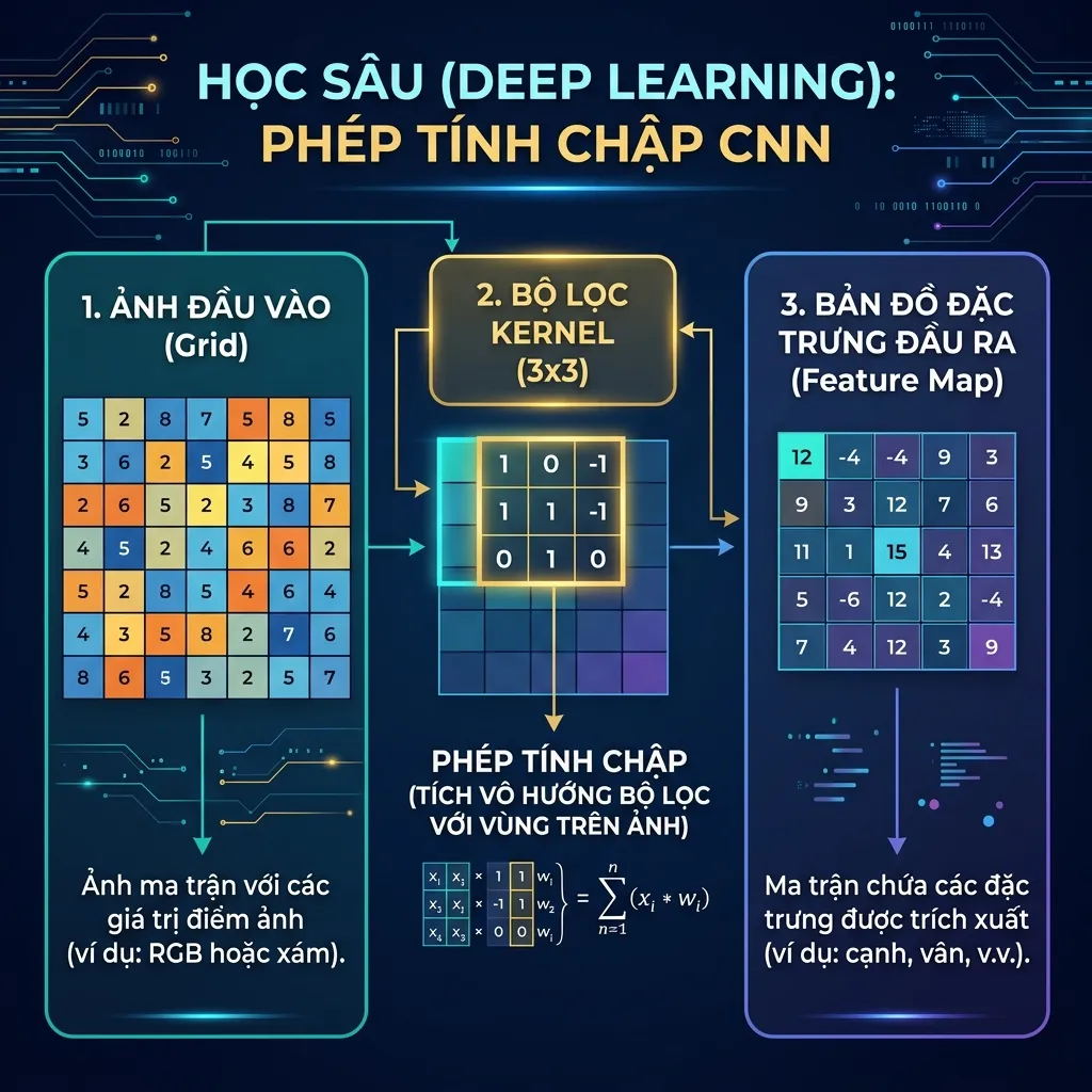
Illustration of Convolution: the filter slides over the image to create a feature map

Input image (6×6):     Filter (3×3):     Feature map (4×4):
┌─────────────────┐    ┌─────────┐       ┌─────────────┐
│ 1 1 1 │ 0 0 0  │    │ 1  0  1 │       │ 4  3  2  1  │
│ 1 1 1 │ 0 0 0  │  × │ 0  1  0 │   =   │ ...         │
│ 1 1 1 │ 0 0 0  │    │ 1  0  1 │       │ ...         │
│ 0 0 0 │ 1 1 1  │    └─────────┘       │ 1  2  3  4  │
│ 0 0 0 │ 1 1 1  │      ↑ Trượt          └─────────────┘
│ 0 0 0 │ 1 1 1  │      qua ảnh
└─────────────────┘

At each position: multiply correspondingly then add (like dot product!) → 1 number.

3 big advantages of CNN:

Advantages	Explanation	Example
Parameter sharing	The same filter is used for the entire image	1 3×3 filter = only 9 params (instead of thousands)
Local connectivity	Each neuron only sees a small area Detect edges, corners, texture
Translation invariance	Recognize objects no matter where they are	Recognize cats no matter what corner they are in

1.3 CNN Architecture — From pixels to decisions

CNN stacks many layers, from simple features → complex features:

Lớp 1: Phát hiện cạnh (edges) ─── Filter đơn giản
    ↓
Lớp 2: Phát hiện góc, texture ─── Kết hợp cạnh
    ↓
Lớp 3: Phát hiện bộ phận (mắt, mũi, tai) ─── Kết hợp góc + texture
    ↓
Lớp 4: Nhận ra đối tượng (mèo, chó) ─── Kết hợp bộ phận

For example: Cat identification: pixel → edge → triangle (ear) + circle (eye) → "cat"!

import torch
import torch.nn as nn

class SimpleCNN(nn.Module):
    def __init__(self, num_classes=10):
        super().__init__()
        self.features = nn.Sequential(
            # === Lớp 1: Phát hiện đặc trưng cơ bản ===
            nn.Conv2d(1, 32, kernel_size=3, padding=1),  # 28×28 → 28×28, 32 filters
            nn.ReLU(),
            nn.MaxPool2d(2),                              # 28×28 → 14×14 (thu nhỏ)
            
            # === Lớp 2: Phát hiện đặc trưng phức tạp hơn ===
            nn.Conv2d(32, 64, kernel_size=3, padding=1), # 14×14 → 14×14, 64 filters
            nn.ReLU(),
            nn.MaxPool2d(2),                              # 14×14 → 7×7
        )
        self.classifier = nn.Sequential(
            nn.Flatten(),                # 64 × 7 × 7 = 3136 số
            nn.Linear(64 * 7 * 7, 128), # Dense layer
            nn.ReLU(),
            nn.Linear(128, num_classes)  # Output: 10 lớp (0-9)
        )

    def forward(self, x):
        features = self.features(x)      # Trích xuất đặc trưng
        return self.classifier(features)  # Phân loại

# Test
model = SimpleCNN(num_classes=10)
x = torch.randn(8, 1, 28, 28)  # 8 ảnh, 1 kênh (grayscale), 28×28
output = model(x)
print(f"Input: {x.shape} → Output: {output.shape}")  # [8, 10]
print(f"Tổng parameters: {sum(p.numel() for p in model.parameters()):,}")

1.4 Famous CNNs — Historical milestones

Model	Year	Features	Why is it important
LeNet-5	1998	The first pragmatic CNN	Read numbers on bank checks
AlexNet	2012	GPU training, ReLU, Dropout	Wins ImageNet → Deep Learning explodes
VGG	2014	Very deep (16-19 layers), only use 3×3	Proving "deeper = better"
ResNet	2015	Skip connections, 152 classes	Solving vanishing gradients in very deep networks
EfficientNet	2019	Smart Scale	Optimize speed/accuracy

💡 Exercise 1:

Calculate by hand: if the input is a 32×32 image, use filter 5×5, stride=1, no padding → what size is the feature map? Formula: output_size = (input_size - kernel_size) / stride + 1

What if we add padding=2?

Why does MaxPool2d(2) reduce image size by 1/2?

2. Sequence Data Problem — "Sequence matters"

CNNs are great for images, but what about sequential data (text, speech, time series)?

2.1 Why is a different architecture needed?

Example 1 — Order of meaning change:

"Tôi KHÔNG thích pizza"  ≠  "Tôi thích pizza"
→ Từ "không" ở giữa thay đổi nghĩa TOÀN CÂU

Example 2 — Distant context:

"Người phụ nữ mặc áo đỏ, đeo kính, cầm ô,
 đứng cạnh cây cổ thụ trong công viên,
 đang ____ với con chó."
→ Cần nhớ "người phụ nữ" từ đầu câu để điền đúng!

Example 3 — Variable length:

Input 1: "Xin chào" (2 từ)
Input 2: "Hôm nay trời đẹp quá, chúng ta đi dạo nhé!" (9 từ)
→ MLP cần input cố định → không xử lý được!

CNN can handle short text (TextCNN), but it is difficult to capture distant relationships between words at the beginning and end of long sentences.

💡 Exercise 2: Think of 2 more Vietnamese examples where the word order completely changes the meaning. Suggestions: negative, passive sentences...

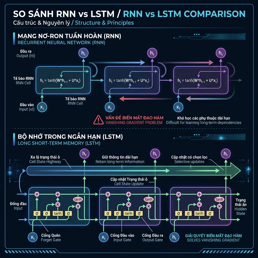
3. Recurrent Neural Networks (RNN) — "Read every word, remember it in your head"

3.1 Main idea

Everyday life example: You read a novel. You read page by page, and after each page, you remember what you read (hidden state). New page + old memories → new understanding.

RNN works exactly the same: reads every word, maintaining a hidden state (short-term memory) that is updated at each step:

     x₁ ("Con")    x₂ ("mèo")    x₃ ("đang")    x₄ ("ngủ")
       ↓              ↓              ↓               ↓
h₀ → [RNN] → h₁ → [RNN] → h₂ → [RNN] → h₃ → [RNN] → h₄
 ↑            ↑             ↑             ↑            ↑
(ban đầu    (nhớ          (nhớ          (nhớ         (nhớ toàn
 trống)     "Con")        "Con mèo")    "Con mèo     câu)
                                         đang")

h_t = tanh(W_hh × h_{t-1} + W_xh × x_t + b)
       ↑           ↑              ↑
   activation   ký ức cũ       từ mới

class SimpleRNN(nn.Module):
    def __init__(self, input_size, hidden_size, output_size):
        super().__init__()
        self.hidden_size = hidden_size
        self.rnn = nn.RNN(input_size, hidden_size, batch_first=True)
        self.fc = nn.Linear(hidden_size, output_size)

    def forward(self, x):
        # x: (batch, seq_len, input_size) — batch câu, mỗi câu là chuỗi
        out, hidden = self.rnn(x)
        # Dùng hidden state cuối (chứa ký ức toàn câu) để dự đoán
        return self.fc(hidden.squeeze(0))

# Ví dụ: phân loại câu positive/negative
rnn = SimpleRNN(input_size=128, hidden_size=256, output_size=2)
x = torch.randn(8, 20, 128)  # 8 câu, mỗi câu 20 từ, mỗi từ embedding 128
output = rnn(x)
print(f"Input: {x.shape} → Output: {output.shape}")  # [8, 2]

3.2 Vanishing Gradient — Fatal weakness

Normal life example: You play the "Telephone game" — 20 people line up, the first person whispers a sentence, passing it on to each person. By the last person, the information was completely distorted because it went through too many steps.

Same goes for RNN! When backpropagation over multiple time steps, the gradient is multiplied successively by the same matrix W:

∂L/∂h₀ = ∂L/∂h_T × (W)^T lần

Case	Consequences	Numerical example
\|W\| < 1	gradient → 0 (vanishing)	0.9^20 = 0.12 → almost lost!
\|W\| > 1	gradient → ∞ (exploding)	1.1^20 = 6.7 → boom!

Practical consequences: Basic RNN only remembers ~10-20 most recent words. With a sentence 100 words long, RNN completely "forgot" the beginning of the sentence.

# Demo: gradient vanishing qua nhiều bước nhân
w = 0.9  # < 1
gradients = [w**t for t in range(20)]
print("Gradient từ t=0 đến t=19:")
print([f"{g:.4f}" for g in gradients])
# [1.0, 0.9, 0.81, 0.729, ..., 0.1351] → giảm 87%!

print(f"\nSau 20 bước: gradient chỉ còn {gradients[-1]:.1%} ban đầu")
print(f"Sau 50 bước: {0.9**50:.6f} → gần như = 0!")

💡 Exercise 3:

If W = 1.1 instead of 0.9, what is the gradient after 20 steps? After 100 steps?

Why does gradient clipping (limit the gradient between [-max, max]) help solve exploding but NOT vanishing?

4. Long Short-Term Memory (LSTM) — "Selective memory"

4.1 Main idea

Real life example: Compare RNN vs LSTM:

RNN = note on small Post-it → can only write a little, new writing over old
LSTM = note on locked notebook → possible:
- Delete old information you don't need (forget gate) — "delete page"
- Added important new information (input gate) — "write new page"
- Read information needed (output gate) — "open page to read"

Compare RNN vs LSTM architecture with cell state and 3 gates

4.2 Three gates of LSTM

LSTM maintains 2 streams of information:

Cell state (C) = "notebook" — long-term memory, running throughout the chain like a conveyor belt
Hidden state (h) = "Post-it" — short-term memory, used for the current step

Forget Gate:  f_t = σ(W_f · [h_{t-1}, x_t] + b_f)    ← "Quên gì?"
Input Gate:   i_t = σ(W_i · [h_{t-1}, x_t] + b_i)    ← "Nhớ gì mới?"
              C̃_t = tanh(W_C · [h_{t-1}, x_t] + b_C)  ← "Thông tin mới"
Cell Update:  C_t = f_t × C_{t-1} + i_t × C̃_t         ← "Cập nhật sổ tay"
Output Gate:  o_t = σ(W_o · [h_{t-1}, x_t] + b_o)     ← "Output gì?"
              h_t = o_t × tanh(C_t)                     ← "Đọc & xuất"

Concrete example — LSTM reads the sentence "I was born in Vietnam. I studied at university in the US for 4 years. My native language is ___":

Step	Forget gates	Input gate	Cell state
"Vietnam"	Keep it all	Write "nationality: VN"	{nationality: VN}
"America"	Keep VN (don't forget!)	Write "study abroad: USA"	{nationality: Vietnamese, studying abroad: USA}
"4 years"	Keep it all	Write "time: 4 years"	{nationality: VN, study abroad: US, 4 years}
"mother..."	Forget "study abroad"	Focus on "nationality"	→ Output: "Vietnamese" ✅

4.3 Code LSTM — Emotion classification

class SentimentLSTM(nn.Module):
    def __init__(self, vocab_size, embed_dim, hidden_size, n_layers=2):
        super().__init__()
        self.embedding = nn.Embedding(vocab_size, embed_dim, padding_idx=0)
        self.lstm = nn.LSTM(
            embed_dim, hidden_size,
            num_layers=n_layers,     # 2 lớp LSTM xếp chồng
            batch_first=True,
            dropout=0.3,             # Chống overfit
            bidirectional=True       # Đọc cả 2 chiều!
        )
        self.fc = nn.Linear(hidden_size * 2, 1)  # ×2 vì bidirectional
        self.sigmoid = nn.Sigmoid()

    def forward(self, x):
        embedded = self.embedding(x)           # Token IDs → vectors
        lstm_out, (hidden, _) = self.lstm(embedded)
        # Lấy hidden state cuối của cả 2 chiều (forward + backward)
        hidden = torch.cat([hidden[-2], hidden[-1]], dim=1)
        return self.sigmoid(self.fc(hidden))   # 0→1: negative→positive

# Ví dụ sử dụng
model = SentimentLSTM(vocab_size=10000, embed_dim=128, hidden_size=256)
x = torch.randint(0, 10000, (8, 50))  # 8 câu, mỗi câu 50 tokens
output = model(x)
print(f"Sentiment predictions: {output.squeeze()[:3]}")  # 3 câu đầu

Bidirectional LSTM = bidirectional reading (left→right AND right→left). Why? Because sometimes you need to look also behind to understand the meaning:

"Anh ấy không phải là người ____ nhất, nhưng rất chăm chỉ"
→ Cần đọc "nhưng rất chăm chỉ" (phía sau) để biết ____ = "giỏi" (chứ không phải "tệ")

4.4 Compare RNN vs LSTM vs GRU

	RNN	LSTM	GRU
Gates	0	3 (forget, input, output)	2 (reset, update)
Parameters	At least	Most	Average
Remember far	❌ ~10 words	✅ ~200 words	✅ ~200 words
Train speed	Fast	Slow	Average
When to use	Demo/learning	Long text, NLP	Long text, little data

GRU is a simplified version of LSTM: combine forget + input gate into update gate, remove cell state. Performance is equivalent to LSTM but with fewer parameters.

💡 Exercise 4:

How many weight matrices does LSTM have? Hint: each gate has 2 matrices (W for input, U for hidden state), plus cell state candidate.

If hidden_size = 256, input_size = 128, total parameters of 1 LSTM cell = ? Formula: 4 × (input_size × hidden_size + hidden_size × hidden_size + hidden_size)

5. Limitations of LSTM and why do we need a Transformer

Although LSTM is much more powerful than RNN, it still has 2 fundamental problems that created the Transformer revolution:

5.1 ❌ Sequential Processing — "One word at a time"

x₁ → h₁ → x₂ → h₂ → x₃ → h₃ → ... → x_1000 → h_1000
     ↑ phải chờ ↑ phải chờ ↑ phải chờ

LSTM must process sequentially — h₃ depends on h₂, h₂ depends on h₁. This means:

Consequences	Explanation	Influence
Not parallelized	GPU has 10,000 cores but only uses 1	Wasting 99.99% GPU
Slow Training	Sentence 1000 words = 1000 sequential steps	Day → week → month
Cannot scale	2x long = 2x slow (linear)	Unable to process long books/documents

Example: Train LSTM on 1 million sentences × 100 words = 100 million sequential steps. Transformer can process parallel = 100× faster!

5.2 ❌ Information Bottleneck — "Information Bottleneck"

Although cell state helps to remember further, all meaning of a sentence must "pass through" a vector h_T of a fixed size (e.g. 256 numbers):

"The cat that ate the mouse that lived in the house that Jack built sat on the mat"
                                                                      ↓
                                                              h_T = [0.2, -0.3, ...]
                                                              (nén 15 từ → 256 số!)

For a 1000 word sentence, the 256-digit vector is not enough to remember everything → information is lost.

5.3 ✅ Solution: Transformer (2017)

Transformer solves both problems with Attention Mechanism:

LSTM problem	Transformer Solutions
Sequential processing	Parallelization — process all words at once
Information bottleneck	Attention — each word "looks directly" at every other word

LSTM: x₁ → x₂ → x₃ → x₄ → x₅  (tuần tự, chậm)

Transformer:
x₁ ←→ x₂     
x₁ ←→ x₃     Tất cả từ "nhìn" nhau
x₁ ←→ x₄     cùng lúc, song song!
x₂ ←→ x₃     
...

This is the breakthrough of the article "Attention Is All You Need" (2017) — completely replacing RNN/LSTM with attention mechanism. We will go deeper in the next article.

💡 Exercise 5:

LSTM processes a 100-word sentence in 100 steps. How many steps does the Transformer require? (Hint: Transformer processes all words in parallel)

Why does Transformer have a "quadratic attention cost" problem? Hint: if there are N words, how many other words must each word "see"?

6. When should I still use CNN/RNN/LSTM?

Although Transformer dominates NLP, CNN and LSTM still have a place in many problems:

CNN is still used for:

Computer Vision: ResNet, EfficientNet are still popular (although Vision Transformer is replacing)
Audio processing: 1D convolution for audio classification
Simple Text classification: TextCNN is fast, lightweight, and highly accurate for small problems
Edge devices: Lightweight CNN that can run on phones (MobileNet)

LSTM/GRU is still used for:

Time series on small devices: predicting sensor data on IoT
Streaming data: data arrives continuously (not in batches)
Small Dataset: Transformer is easy to overfit with little data, LSTM is better
Real-time inference: LSTM processes each step, response is fast

Rule: If there is a lot of data + powerful GPU → Transformer. If little data + small device → CNN/LSTM.

💡 Exercise 6: Given 3 problems, which architecture would you choose? Explanation:

Classify spam/ham emails (1000 emails, each email ~50 words)

Chatbot answers questions (1 million conversations)

Facial recognition on security cameras (real-time)

Summary

Architecture	Strong	Weak	Used for	Golden Age
CNN	Local patterns, fast	Long-range, sequence	Image, short text	2012–present
RNN	Sequential processing	Vanishing gradient	Simple sequences	2013–2017
LSTM	Long-range memory	Sequential, slow	Medium sequences	2015–2018
Transformer	Parallel, long-range	Cost O(N²)	NLP, LLM, Vision	2017–present

Evolutionary timeline

1998: LeNet (CNN cho chữ số)
  ↓
2012: AlexNet (CNN thắng ImageNet → Deep Learning bùng nổ)
  ↓
2014: Sequence-to-Sequence (LSTM cho dịch thuật)
  ↓
2015: Attention + LSTM (cải thiện dịch thuật)
  ↓
2017: "Attention Is All You Need" → TRANSFORMER 💥
  ↓
2018: BERT, GPT-1 (Transformer thống trị NLP)
  ↓
2020+: GPT-3, ChatGPT → LLM thời đại mới

General exercises

✅ Complete all small exercises in each section (1, 2, 3, 4, 5, 6)
Using PyTorch, implement SimpleCNN in section 1.3 and train on the MNIST dataset. Achieving >98% accuracy.
Implement SentimentLSTM in section 4.3 and train on movie reviews dataset (IMDB). Achieving >85% accuracy.
Experimental comparison: Train the same text classification problem with (a) MLP, (b) CNN (TextCNN), (c) LSTM. Compare accuracy, training time, and number of parameters.
Read the abstract of the article "Attention Is All You Need" — lists 3 reasons the author gives for replacing RNN with Transformer.

Next article: We will learn about the Attention mechanism — the key to the extraordinary power of Transformer and all modern LLMs.

Lesson 4: Deep Learning Overview — CNN, RNN, LSTM