1. Introduction: Why Is U-Net the Heart of Diffusion Models?
In the previous lesson, you understood that the forward process adds noise to images at each timestep. Now the question is: which model will learn to denoise — that is, reverse this process? The answer is U-Net.
U-Net was originally designed for image segmentation in medical imaging (2015, Ronneberger et al.). Its special architecture — encoder-decoder with skip connections — helps preserve spatial details while learning features at multiple levels of abstraction. This is exactly what diffusion models need.
Exam tip: In the assessment, you will have to implement U-Net from scratch. Understanding tensor dimensions through each layer is the key. NVIDIA DLI requires you to write working code, not just understand theory.
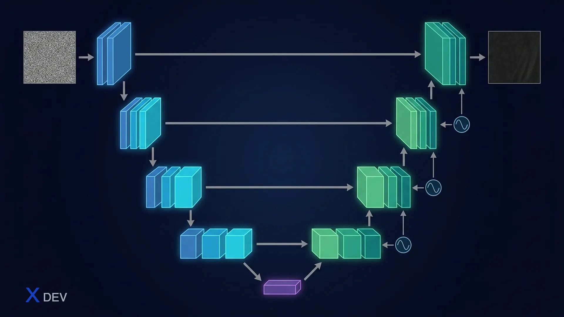
2. U-Net Architecture: Encoder-Decoder with Skip Connections
2.1 Architecture Overview
U-Net has a "U" shape with 3 main parts:
- Encoder (Contracting Path): reduces spatial resolution, increases channels — learns high-level abstract features
- Bottleneck: smallest spatial, largest channels — captures global context
- Decoder (Expanding Path): increases spatial resolution, decreases channels — recovers details
- Skip Connections: directly connect encoder features to corresponding decoder — preserves fine-grained details
U-Net Architecture for Diffusion (input 64×64×1)
═══════════════════════════════════════════════

          ENCODER                              DECODER
     (Contracting Path)                   (Expanding Path)

  ┌─────────────────┐                 ┌─────────────────┐
  │  64 × 64 × 1    │   Input Image   │  64 × 64 × 1    │  Output (denoised)
  └────────┬────────┘                 └────────▲────────┘
           │                                    │
           ▼                                    │
  ┌─────────────────┐  skip connection  ┌─────────────────┐
  │  64 × 64 × 64   │ ───────────────► │  64 × 64 × 64   │  UpBlock + Concat
  │  Conv→GN→GELU   │   (concatenate)   │  Conv→GN→GELU   │
  └────────┬────────┘                 └────────▲────────┘
           │ Downsample                        │ Upsample
           ▼                                    │
  ┌─────────────────┐  skip connection  ┌─────────────────┐
  │  32 × 32 × 128  │ ───────────────► │  32 × 32 × 128  │  UpBlock + Concat
  │  Conv→GN→GELU   │   (concatenate)   │  Conv→GN→GELU   │
  └────────┬────────┘                 └────────▲────────┘
           │ Downsample                        │ Upsample
           ▼                                    │
  ┌─────────────────┐  skip connection  ┌─────────────────┐
  │  16 × 16 × 256  │ ───────────────► │  16 × 16 × 256  │  UpBlock + Concat
  │  Conv→GN→GELU   │   (concatenate)   │  Conv→GN→GELU   │
  └────────┬────────┘                 └────────▲────────┘
           │ Downsample                        │ Upsample
           ▼                                    │
  ┌──────────────────────────────────────────────┐
  │              8 × 8 × 512                      │
  │           BOTTLENECK                          │
  │     Conv → GN → GELU → Conv → GN             │
  │  (smallest spatial, largest channels)         │
  └───────────────────────────────────────────────┘

  + Timestep Embedding ──► injected into EVERY ResidualBlock via linear projection
2.2 Encoder Path (Contracting)
Each encoder level performs:
- Convolution: 3×3 conv with padding=1 (preserves spatial size)
- Group Normalization: normalizes by groups instead of batch
- GELU Activation: smoother non-linearity than ReLU
- Downsample: reduces spatial resolution by 2× (can use stride=2 conv or Rearrange Pooling)
At each level, channels double and spatial halves. For example:
| Level | Input Shape | Output Shape | Operation |
|---|---|---|---|
| 0 | B × 1 × 64 × 64 | B × 64 × 64 × 64 | Initial Conv |
| 1 | B × 64 × 64 × 64 | B × 128 × 32 × 32 | ResBlock → Down |
| 2 | B × 128 × 32 × 32 | B × 256 × 16 × 16 | ResBlock → Down |
| 3 | B × 256 × 16 × 16 | B × 512 × 8 × 8 | ResBlock → Down |
2.3 Decoder Path (Expanding)
Opposite to the encoder, the decoder increases spatial and decreases channels:
- Upsample: increases spatial resolution by 2× (typically using
nn.Upsampleornn.ConvTranspose2d) - Concatenate with skip connection from the encoder at the same level
- Convolution → GroupNorm → GELU: process concatenated features
Exam tip: When concatenating skip connections, the number of channels temporarily doubles. For example: upsample output has 256 channels + skip has 256 channels = 512 channels input to conv. This is a common implementation error — pay attention to
in_channelsof the conv after concat!
2.4 Skip Connections — Why Are They Important?
Without skip connections, the decoder must "guess" all spatial details from only the 8×8 bottleneck — nearly impossible. Skip connections enable:
- Gradient flow: gradients flow directly from the loss back to deep encoder layers — easier training
- Detail preservation: high-level encoder retains edges and textures — decoder reuses them instead of relearning
- Multi-scale features: decoder receives both high-level (from bottleneck) and low-level (from skip) features
3. Key Components: GroupNorm, GELU, Rearrange Pooling
3.1 Group Normalization
In diffusion models, batch size is usually very small (4-8) because each image consumes a lot of GPU memory. Batch Normalization performs poorly with small batches because statistics (mean, variance) computed over the batch are unstable.
Group Normalization solves this by dividing channels into groups and normalizing within each group, for each sample independently — independent of batch size.
Group Normalization vs Batch Normalization
══════════════════════════════════════════

Batch Normalization:              Group Normalization:
  normalize across N (batch)        normalize within groups of C

  ┌───┬───┬───┬───┐               ┌───┬───┬───┬───┐
  │ N │   │   │   │               │   │   │   │   │  N (batch)
  ├───┼───┼───┼───┤               ├───┼───┼───┼───┤
  │   │   │   │   │  C            │ G1│ G1│ G2│ G2│  C (channels)
  ├───┼───┼───┼───┤  (channels)   ├───┼───┼───┼───┤  split into groups
  │   │   │   │   │               │ G1│ G1│ G2│ G2│
  ├───┼───┼───┼───┤               ├───┼───┼───┼───┤
  │   │   │   │   │  H×W          │   │   │   │   │  H×W
  └───┴───┴───┴───┘               └───┴───┴───┴───┘
     ▲                                 ▲
     normalize column (across N)       normalize block (within group)
     ⚠ small batch → unstable          ✓ independent of batch size
import torch.nn as nn

# GroupNorm: split 64 channels into 8 groups (8 channels per group)
norm = nn.GroupNorm(num_groups=8, num_channels=64)

# With input shape (B, 64, 32, 32):
# - Split 64 channels into 8 groups, 8 channels each
# - Compute mean, var over (8, 32, 32) = 8192 elements per group per sample
# - Normalize independently for each sample, each group

x = torch.randn(4, 64, 32, 32)
out = norm(x)  # shape: (4, 64, 32, 32) — shape unchanged
| Feature | BatchNorm | GroupNorm | LayerNorm | InstanceNorm |
|---|---|---|---|---|
| Normalizes across | Batch (N) | Channel groups | All channels | Each channel |
| Batch size dependency | Yes ⚠ | No ✓ | No ✓ | No ✓ |
| Small batch performance | Poor | Good | OK | OK |
| Use case | Classification | Diffusion, Detection | Transformers (NLP) | Style Transfer |
| PyTorch API | nn.BatchNorm2d(C) | nn.GroupNorm(G, C) | nn.LayerNorm(shape) | nn.InstanceNorm2d(C) |
3.2 GELU Activation
GELU (Gaussian Error Linear Unit) is the standard activation function in modern models (Transformers, Diffusion Models). Unlike the "hard" ReLU (clips negatives to 0), GELU is smooth and allows a portion of negative values to "leak" through.
Formula: GELU(x) = x · Φ(x), where Φ(x) is the CDF of the standard normal distribution.
Activation Functions Comparison
═══════════════════════════════

 Output                              Output
   │     ReLU                          │     GELU
   │      ╱                            │      ╱
   │     ╱                             │    ╱
   │    ╱                              │  ╱
───┼───╱────── Input            ───┼──╱─────── Input
   │  ╱                              ╱│
   │ ╱                              ╱ │
   │╱  (hard cutoff at 0)         ╱  │  (smooth curve, allows
   │                             ╱    │   small negative values)

 ReLU(x) = max(0, x)           GELU(x) = x · Φ(x)
 ⚠ Dead neurons problem         ✓ Smoother gradient flow
 ⚠ Not differentiable at 0      ✓ Better for deep networks
import torch.nn as nn

# Method 1: use module
activation = nn.GELU()
out = activation(x)

# Method 2: use functional
import torch.nn.functional as F
out = F.gelu(x)

# Method 3: approximate (faster, used in DLI course)
activation = nn.GELU(approximate='tanh')
3.3 Rearrange Pooling (Space-to-Channel)
Rearrange Pooling is a downsampling technique that replaces MaxPool/AvgPool. Instead of discarding information (MaxPool picks max, AvgPool takes average), Rearrange "folds" spatial dimensions into the channel dimension — retaining all information.
Rearrange Pooling: (B, C, 2H, 2W) → (B, 4C, H, W)
════════════════════════════════════════════════════

Input: (B, C, 4, 4)                   Output: (B, 4C, 2, 2)

Channel c:                             4 channels (each is 1 "position"):
┌───┬───┬───┬───┐                     Channel c_0:    Channel c_1:
│ a │ b │ e │ f │                     ┌───┬───┐       ┌───┬───┐
├───┼───┼───┼───┤                     │ a │ e │       │ b │ f │
│ c │ d │ g │ h │      ────►         ├───┼───┤       ├───┼───┤
├───┼───┼───┼───┤   Rearrange        │ i │ m │       │ j │ n │
│ i │ j │ m │ n │                     └───┴───┘       └───┴───┘
├───┼───┼───┼───┤
│ k │ l │ o │ p │                     Channel c_2:    Channel c_3:
└───┴───┴───┴───┘                     ┌───┬───┐       ┌───┬───┐
                                       │ c │ g │       │ d │ h │
Spatial: 4×4, Channels: C             ├───┼───┤       ├───┼───┤
                                       │ k │ o │       │ l │ p │
                                       └───┴───┘       └───┴───┘

                                       Spatial: 2×2, Channels: 4C
                                       ✓ NO information loss!
from einops import rearrange

def rearrange_downsample(x):
    """Downsample by rearranging spatial dims into channels.
    (B, C, H, W) -> (B, 4C, H/2, W/2)
    """
    return rearrange(x, 'b c (h p1) (w p2) -> b (c p1 p2) h w', p1=2, p2=2)

# Example:
x = torch.randn(2, 64, 32, 32)
out = rearrange_downsample(x)
print(out.shape)  # torch.Size([2, 256, 16, 16])

# Without einops, using pure PyTorch:
def rearrange_downsample_pure(x):
    B, C, H, W = x.shape
    x = x.reshape(B, C, H // 2, 2, W // 2, 2)
    x = x.permute(0, 1, 3, 5, 2, 4)  # (B, C, 2, 2, H/2, W/2)
    x = x.reshape(B, C * 4, H // 2, W // 2)
    return x
| Downsampling Method | Information Loss | Channel Change | Use in Diffusion |
|---|---|---|---|
| MaxPool2d | High (keeps only max) | Unchanged | Rarely used |
| AvgPool2d | Medium (takes average) | Unchanged | Rarely used |
| Stride-2 Conv | Learned (trainable) | Configurable | Common |
| Rearrange Pooling | None ✓ | ×4 | NVIDIA DLI course ✓ |
Exam tip: NVIDIA DLI uses Rearrange Pooling instead of MaxPool. In the assessment, you may need to implement this function using
einops.rearrangeor pure PyTorch (reshape+permute). Remember that channels increase 4 times when spatial decreases 2× in each dimension.
4. Sinusoidal Position Embeddings for Timestep
4.1 Why Do We Need Timestep Embedding?
U-Net needs to know which timestep it's at in the diffusion process to denoise appropriately:
- Large timestep (t near T): image is nearly pure noise → model needs to recover overall structure
- Small timestep (t near 0): image is nearly clean → model only needs to refine small details
We convert the integer timestep t into a continuous embedding vector of length embed_dim, injected into every layer of the U-Net.
4.2 Sinusoidal Embedding Formula
Identical to Positional Encoding in Transformer ("Attention Is All You Need"):
PE(t, 2i)   = sin(t / 10000^(2i/d))
PE(t, 2i+1) = cos(t / 10000^(2i/d))

Where:
  t = timestep (integer: 0, 1, 2, ..., T)
  d = embedding dimension (e.g., 128)
  i = index in embedding vector (0, 1, 2, ..., d/2 - 1)

Example with d=8:
  PE(t) = [sin(t/1), cos(t/1), sin(t/100), cos(t/100),
           sin(t/10000), cos(t/10000), sin(t/1000000), cos(t/1000000)]

  → Low frequency terms (end): change slowly → encode "big picture" timestep
  → High frequency terms (start): change rapidly → encode fine timestep differences
4.3 Implement TimestepEmbedding
import torch
import torch.nn as nn
import math

class SinusoidalPositionEmbedding(nn.Module):
    """Convert integer timestep to sinusoidal embedding vector."""

    def __init__(self, embed_dim):
        super().__init__()
        self.embed_dim = embed_dim

    def forward(self, timesteps):
        """
        Args:
            timesteps: (B,) — integer timesteps
        Returns:
            embeddings: (B, embed_dim) — sinusoidal embeddings
        """
        device = timesteps.device
        half_dim = self.embed_dim // 2

        # Compute frequencies: 1/10000^(2i/d) for i = 0, 1, ..., d/2-1
        exponent = torch.arange(half_dim, device=device).float() / half_dim
        freqs = torch.exp(-math.log(10000.0) * exponent)  # shape: (d/2,)

        # Multiply timestep by frequencies: (B, 1) * (1, d/2) = (B, d/2)
        args = timesteps[:, None].float() * freqs[None, :]

        # Concat sin and cos: (B, d/2) cat (B, d/2) = (B, d)
        embeddings = torch.cat([torch.sin(args), torch.cos(args)], dim=-1)

        return embeddings  # shape: (B, embed_dim)


class TimestepMLPEmbedding(nn.Module):
    """Sinusoidal embedding + MLP projection (used in DLI course)."""

    def __init__(self, embed_dim, hidden_dim=None):
        super().__init__()
        if hidden_dim is None:
            hidden_dim = embed_dim * 4

        self.sinusoidal = SinusoidalPositionEmbedding(embed_dim)
        self.mlp = nn.Sequential(
            nn.Linear(embed_dim, hidden_dim),
            nn.GELU(),
            nn.Linear(hidden_dim, hidden_dim),
        )

    def forward(self, timesteps):
        """
        Args:
            timesteps: (B,) — integer timesteps
        Returns:
            (B, hidden_dim) — projected timestep embeddings
        """
        x = self.sinusoidal(timesteps)  # (B, embed_dim)
        x = self.mlp(x)                 # (B, hidden_dim)
        return x
4.4 Injecting Timestep into U-Net
The timestep embedding is injected into every ResidualBlock by:
- Projecting the timestep embedding to match the number of channels in the feature map (using
nn.Linear) - Reshaping to
(B, C, 1, 1)for broadcasting - Adding to the feature map after the first GroupNorm
Timestep Injection Flow
═══════════════════════

timestep t ──► SinusoidalEmbed ──► MLP ──► t_emb (B, hidden_dim)
                                              │
                                    Linear(hidden_dim, C)
                                              │
                                         (B, C, 1, 1)   ← reshape for broadcasting
                                              │
Feature Map: ─── Conv ─── GroupNorm ────── (+) ────── GELU ─── Conv ─── ...
                                          add here
Exam tip: The timestep embedding is added, not concatenated, to the feature map. Injection happens after GroupNorm, before GELU in each ResidualBlock. This is a fixed pattern in the DLI course.
5. Build U-Net from Scratch — Step by Step
5.1 ResidualBlock
This is the most fundamental building block. Each ResidualBlock consists of 2 conv layers + GroupNorm + GELU, plus a residual connection and timestep injection.
class ResidualBlock(nn.Module):
    """Residual block with timestep embedding injection.

    Flow: x → Conv1 → GN1 → (+t_emb) → GELU → Conv2 → GN2 → GELU → (+residual) → out
    """

    def __init__(self, in_channels, out_channels, time_emb_dim):
        super().__init__()

        # First conv layer
        self.conv1 = nn.Conv2d(in_channels, out_channels, kernel_size=3, padding=1)
        self.norm1 = nn.GroupNorm(num_groups=8, num_channels=out_channels)

        # Second conv layer
        self.conv2 = nn.Conv2d(out_channels, out_channels, kernel_size=3, padding=1)
        self.norm2 = nn.GroupNorm(num_groups=8, num_channels=out_channels)

        # Activation
        self.act = nn.GELU()

        # Timestep embedding projection: project to out_channels
        self.time_mlp = nn.Sequential(
            nn.GELU(),
            nn.Linear(time_emb_dim, out_channels),
        )

        # Residual connection: if in_channels != out_channels, need 1x1 conv
        if in_channels != out_channels:
            self.residual_conv = nn.Conv2d(in_channels, out_channels, kernel_size=1)
        else:
            self.residual_conv = nn.Identity()

    def forward(self, x, t_emb):
        """
        Args:
            x: (B, in_channels, H, W) — input feature map
            t_emb: (B, time_emb_dim) — timestep embedding
        Returns:
            (B, out_channels, H, W)
        """
        residual = self.residual_conv(x)   # (B, out_channels, H, W)

        # First layer
        h = self.conv1(x)                   # (B, out_channels, H, W)
        h = self.norm1(h)                   # normalize

        # Inject timestep embedding
        t = self.time_mlp(t_emb)            # (B, out_channels)
        t = t[:, :, None, None]             # (B, out_channels, 1, 1) broadcast
        h = h + t                           # add timestep info

        h = self.act(h)                     # GELU activation

        # Second layer
        h = self.conv2(h)                   # (B, out_channels, H, W)
        h = self.norm2(h)                   # normalize
        h = self.act(h)                     # GELU activation

        return h + residual                  # residual connection
5.2 DownBlock (Encoder Level)
class DownBlock(nn.Module):
    """Encoder block: ResidualBlock + Rearrange Downsample."""

    def __init__(self, in_channels, out_channels, time_emb_dim):
        super().__init__()
        self.res_block = ResidualBlock(in_channels, out_channels, time_emb_dim)

    def downsample(self, x):
        """Rearrange pooling: (B, C, H, W) -> (B, 4C, H/2, W/2)"""
        B, C, H, W = x.shape
        x = x.reshape(B, C, H // 2, 2, W // 2, 2)
        x = x.permute(0, 1, 3, 5, 2, 4).reshape(B, C * 4, H // 2, W // 2)
        return x

    def forward(self, x, t_emb):
        """
        Args:
            x: (B, in_channels, H, W)
            t_emb: (B, time_emb_dim)
        Returns:
            skip: (B, out_channels, H, W) — for skip connection
            down: (B, out_channels*4, H/2, W/2) — downsampled for next level
        """
        skip = self.res_block(x, t_emb)    # (B, out_channels, H, W)
        down = self.downsample(skip)         # (B, out_channels*4, H/2, W/2)
        return skip, down
5.3 UpBlock (Decoder Level)
class UpBlock(nn.Module):
    """Decoder block: Upsample + Concat skip + ResidualBlock."""

    def __init__(self, in_channels, skip_channels, out_channels, time_emb_dim):
        super().__init__()
        # in_channels = channels from below level after upsample
        # After concat with skip: in_channels + skip_channels
        self.res_block = ResidualBlock(
            in_channels + skip_channels, out_channels, time_emb_dim
        )
        self.upsample = nn.Upsample(scale_factor=2, mode='nearest')

    def forward(self, x, skip, t_emb):
        """
        Args:
            x: (B, in_channels, H, W) — from below level
            skip: (B, skip_channels, 2H, 2W) — skip connection from encoder
            t_emb: (B, time_emb_dim)
        Returns:
            (B, out_channels, 2H, 2W)
        """
        x = self.upsample(x)               # (B, in_channels, 2H, 2W)
        x = torch.cat([x, skip], dim=1)     # (B, in_channels+skip_channels, 2H, 2W)
        x = self.res_block(x, t_emb)        # (B, out_channels, 2H, 2W)
        return x
5.4 Full U-Net Assembly
class UNet(nn.Module):
    """Complete U-Net for diffusion denoising.

    Architecture: 64×64×1 → encoder (3 levels) → bottleneck → decoder (3 levels) → 64×64×1
    Channel progression: 1 → 64 → 128 → 256 → 512 (bottleneck) → 256 → 128 → 64 → 1
    """

    def __init__(self, in_channels=1, base_channels=64, time_emb_dim=128):
        super().__init__()

        # Timestep embedding
        self.time_embed = TimestepMLPEmbedding(
            embed_dim=time_emb_dim,
            hidden_dim=time_emb_dim * 4
        )
        t_dim = time_emb_dim * 4  # output dim of MLP

        # Initial convolution: 1 → 64
        self.init_conv = nn.Conv2d(in_channels, base_channels, kernel_size=3, padding=1)

        # Encoder path
        # Level 1: 64ch, 64×64 → Rearrange → 256ch, 32×32
        self.down1 = DownBlock(base_channels, base_channels, t_dim)        # 64 → 64 (skip), 256 (down)

        # Level 2: 256ch, 32×32 → Rearrange → 512ch, 16×16
        # Need 1x1 conv before because Rearrange creates 4× channels
        self.down1_proj = nn.Conv2d(base_channels * 4, base_channels * 2, kernel_size=1)
        self.down2 = DownBlock(base_channels * 2, base_channels * 2, t_dim) # 128 → 128 (skip), 512 (down)

        # Level 3: 512ch, 16×16 → Rearrange → 1024ch, 8×8
        self.down2_proj = nn.Conv2d(base_channels * 8, base_channels * 4, kernel_size=1)
        self.down3 = DownBlock(base_channels * 4, base_channels * 4, t_dim) # 256 → 256 (skip), 1024 (down)

        # Bottleneck: 1024ch, 8×8 → 512ch, 8×8
        self.down3_proj = nn.Conv2d(base_channels * 16, base_channels * 8, kernel_size=1)
        self.bottleneck = ResidualBlock(base_channels * 8, base_channels * 8, t_dim)  # 512 → 512

        # Decoder path
        # Level 3: upsample 512 to 16×16, concat skip(256) → 768 → 256
        self.up3 = UpBlock(base_channels * 8, base_channels * 4, base_channels * 4, t_dim)

        # Level 2: upsample 256 to 32×32, concat skip(128) → 384 → 128
        self.up2 = UpBlock(base_channels * 4, base_channels * 2, base_channels * 2, t_dim)

        # Level 1: upsample 128 to 64×64, concat skip(64) → 192 → 64
        self.up1 = UpBlock(base_channels * 2, base_channels, base_channels, t_dim)

        # Final output: 64 → 1
        self.final_conv = nn.Sequential(
            nn.GroupNorm(8, base_channels),
            nn.GELU(),
            nn.Conv2d(base_channels, in_channels, kernel_size=1),
        )

    def forward(self, x, timesteps):
        """
        Args:
            x: (B, 1, 64, 64) — noisy image
            timesteps: (B,) — integer timesteps
        Returns:
            (B, 1, 64, 64) — predicted clean image (or noise)
        """
        # Timestep embedding
        t_emb = self.time_embed(timesteps)    # (B, t_dim)

        # Initial conv
        x = self.init_conv(x)                 # (B, 64, 64, 64)

        # Encoder
        skip1, x = self.down1(x, t_emb)       # skip1: (B,64,64,64), x: (B,256,32,32)
        x = self.down1_proj(x)                 # (B, 128, 32, 32)

        skip2, x = self.down2(x, t_emb)       # skip2: (B,128,32,32), x: (B,512,16,16)
        x = self.down2_proj(x)                 # (B, 256, 16, 16)

        skip3, x = self.down3(x, t_emb)       # skip3: (B,256,16,16), x: (B,1024,8,8)
        x = self.down3_proj(x)                 # (B, 512, 8, 8)

        # Bottleneck
        x = self.bottleneck(x, t_emb)         # (B, 512, 8, 8)

        # Decoder
        x = self.up3(x, skip3, t_emb)         # (B, 256, 16, 16)
        x = self.up2(x, skip2, t_emb)         # (B, 128, 32, 32)
        x = self.up1(x, skip1, t_emb)         # (B, 64, 64, 64)

        # Final output
        x = self.final_conv(x)                 # (B, 1, 64, 64)
        return x
Verify tensor shapes:
# Verify shapes
model = UNet(in_channels=1, base_channels=64, time_emb_dim=128)
x = torch.randn(2, 1, 64, 64)
t = torch.randint(0, 1000, (2,))
out = model(x, t)
print(f"Input:  {x.shape}")    # torch.Size([2, 1, 64, 64])
print(f"Output: {out.shape}")  # torch.Size([2, 1, 64, 64])
print(f"Params: {sum(p.numel() for p in model.parameters()):,}")
Tensor Shape Flow through U-Net (base_channels=64)
═══════════════════════════════════════════════

Layer                    Shape                  Notes
──────────────────────────────────────────────────────────
Input                    (B, 1, 64, 64)
init_conv                (B, 64, 64, 64)        Conv2d(1, 64)

down1 ResBlock           (B, 64, 64, 64)        skip1 ─────────────────┐
down1 Rearrange          (B, 256, 32, 32)       4× channels            │
down1_proj               (B, 128, 32, 32)       1×1 conv reduce        │
                                                                        │
down2 ResBlock           (B, 128, 32, 32)       skip2 ──────────┐      │
down2 Rearrange          (B, 512, 16, 16)       4× channels     │      │
down2_proj               (B, 256, 16, 16)       1×1 conv reduce │      │
                                                                 │      │
down3 ResBlock           (B, 256, 16, 16)       skip3 ───┐      │      │
down3 Rearrange          (B, 1024, 8, 8)        4× ch    │      │      │
down3_proj               (B, 512, 8, 8)         reduce   │      │      │
                                                          │      │      │
bottleneck               (B, 512, 8, 8)                   │      │      │
                                                          │      │      │
up3 Upsample             (B, 512, 16, 16)                │      │      │
up3 Concat skip3         (B, 768, 16, 16) ◄──────────────┘      │      │
up3 ResBlock             (B, 256, 16, 16)                        │      │
                                                                  │      │
up2 Upsample             (B, 256, 32, 32)                        │      │
up2 Concat skip2         (B, 384, 32, 32) ◄─────────────────────┘      │
up2 ResBlock             (B, 128, 32, 32)                               │
                                                                         │
up1 Upsample             (B, 128, 64, 64)                               │
up1 Concat skip1         (B, 192, 64, 64) ◄────────────────────────────┘
up1 ResBlock             (B, 64, 64, 64)

final_conv               (B, 1, 64, 64)         Output = denoised image
Exam tip: In the assessment, you will need to calculate tensor shapes precisely. Rule to remember: Rearrange → channels ×4, spatial ÷2. After concatenating skip connections, channels = channels from upsample + channels from skip. Write these on scratch paper before coding!
6. Train Denoiser Model
6.1 Simple Denoising Task
Before learning the full diffusion process (multiple timesteps), we start with a simple task:
Add Gaussian noise to images → train U-Net to recover the original image
Simple Denoising Task
═════════════════════

Original Image        Add Noise                Noisy Image        U-Net         Denoised Output
   ┌──────┐          ┌──────┐                  ┌──────┐         ┌─────┐         ┌──────┐
   │ 🖼️   │    +     │ ░░░░ │  noise_level     │ ░🖼️░ │  ────► │U-Net│  ────►  │ 🖼️   │
   │      │          │ ░░░░ │  * N(0,1)        │ ░░░░ │         │     │         │      │
   └──────┘          └──────┘                  └──────┘         └─────┘         └──────┘
      x₀               ε                      x_noisy          predict          x̂₀
                                            = x₀ + σ·ε           x₀

Loss = MSE(x̂₀, x₀) = ‖U-Net(x_noisy, t) - x₀‖²
6.2 Training Loop
import torch
import torch.nn as nn
import torch.optim as optim
from torch.utils.data import DataLoader
from torchvision import datasets, transforms

# Hyperparameters
BATCH_SIZE = 32
LEARNING_RATE = 1e-4
EPOCHS = 50
NOISE_LEVEL = 0.5  # σ: controls how much noise to add
DEVICE = torch.device('cuda' if torch.cuda.is_available() else 'cpu')

# Dataset: MNIST (grayscale 28×28 → resize to 64×64)
transform = transforms.Compose([
    transforms.Resize((64, 64)),
    transforms.ToTensor(),           # [0, 1]
    transforms.Normalize([0.5], [0.5])  # [-1, 1]
])
dataset = datasets.MNIST(root='./data', train=True, transform=transform, download=True)
dataloader = DataLoader(dataset, batch_size=BATCH_SIZE, shuffle=True)

# Model, optimizer, loss
model = UNet(in_channels=1, base_channels=64, time_emb_dim=128).to(DEVICE)
optimizer = optim.Adam(model.parameters(), lr=LEARNING_RATE)
loss_fn = nn.MSELoss()

# Training loop
for epoch in range(EPOCHS):
    total_loss = 0
    for batch_idx, (images, _) in enumerate(dataloader):
        images = images.to(DEVICE)                    # (B, 1, 64, 64)

        # Random timesteps (each sample gets a different timestep)
        timesteps = torch.randint(0, 1000, (images.shape[0],), device=DEVICE)

        # Scale noise level by timestep (simple: linear scaling)
        noise_scales = (timesteps.float() / 1000.0 * NOISE_LEVEL)  # (B,)
        noise_scales = noise_scales[:, None, None, None]             # (B,1,1,1)

        # Add noise
        noise = torch.randn_like(images)                             # (B, 1, 64, 64)
        noisy_images = images + noise_scales * noise                 # (B, 1, 64, 64)

        # Forward pass: predict clean image
        predicted_clean = model(noisy_images, timesteps)             # (B, 1, 64, 64)

        # Loss: MSE between predicted clean and actual clean
        loss = loss_fn(predicted_clean, images)

        # Backward pass
        optimizer.zero_grad()
        loss.backward()
        optimizer.step()

        total_loss += loss.item()

    avg_loss = total_loss / len(dataloader)
    print(f"Epoch [{epoch+1}/{EPOCHS}], Loss: {avg_loss:.6f}")
6.3 Visualize Results
import matplotlib.pyplot as plt

@torch.no_grad()
def visualize_denoising(model, dataloader, noise_level=0.5, num_images=5):
    """Display: Original → Noisy → Denoised."""
    model.eval()
    images, _ = next(iter(dataloader))
    images = images[:num_images].to(DEVICE)

    # Add noise
    timesteps = torch.full((num_images,), 500, device=DEVICE)
    noise = torch.randn_like(images) * noise_level
    noisy = images + noise

    # Denoise
    denoised = model(noisy, timesteps)

    # Plot
    fig, axes = plt.subplots(3, num_images, figsize=(num_images * 3, 9))
    titles = ['Original', 'Noisy', 'Denoised']

    for i in range(num_images):
        for j, (img, title) in enumerate(zip(
            [images[i], noisy[i], denoised[i]], titles
        )):
            ax = axes[j][i]
            # Denormalize: [-1,1] → [0,1]
            img_np = (img.cpu().squeeze() * 0.5 + 0.5).clamp(0, 1).numpy()
            ax.imshow(img_np, cmap='gray')
            ax.set_title(title if i == 0 else '')
            ax.axis('off')

    plt.tight_layout()
    plt.savefig('denoising_results.png', dpi=150)
    plt.show()

visualize_denoising(model, dataloader)
Exam tip: In the assessment, you may need to complete the training loop. Remember 3 important steps: (1) add noise to clean image, (2) forward pass through U-Net with noisy image + timestep, (3) compute MSE loss between predicted and original. Don't forget to pass the timestep to the model!
7. Cheat Sheet — U-Net & Denoising
| Concept | Key Detail | Code/Formula |
|---|---|---|
| U-Net Structure | Encoder → Bottleneck → Decoder + Skip Connections | U-shaped, skip = concatenate |
| GroupNorm | Normalize per group, batch-size independent | nn.GroupNorm(8, channels) |
| GELU | Smooth activation, x·Φ(x) | nn.GELU() |
| Rearrange Pooling | (B,C,2H,2W) → (B,4C,H,W), lossless | rearrange(x, 'b c (h p1) (w p2) → b (c p1 p2) h w', p1=2, p2=2) |
| Sinusoidal Embed | sin/cos at varying frequencies | sin(t/10000^(2i/d)), cos(t/10000^(2i/d)) |
| Timestep Injection | Add to feature maps after GroupNorm | h = h + t_emb[:,:,None,None] |
| ResidualBlock | Conv→GN→(+t)→GELU→Conv→GN→GELU + skip | 2 conv layers + residual + timestep |
| Denoising Loss | MSE between predicted clean & actual clean | MSE(model(x_noisy, t), x_clean) |
| Skip Connection Role | Preserve spatial details, improve gradient flow | torch.cat([upsample, skip], dim=1) |
| Channels after Concat | Channels from upsample + channels from skip | Must match in_channels of next conv |
8. Practice Questions
The questions below simulate the NVIDIA DLI coding assessment. Try coding before checking the answers!
Q1: Implement ResidualBlock with Timestep Injection
Complete the forward method of the ResidualBlock below. The block should apply two conv layers with GroupNorm and GELU, inject the timestep embedding after the first normalization, and add a residual connection.
class ResidualBlock(nn.Module):
    def __init__(self, in_ch, out_ch, t_dim):
        super().__init__()
        self.conv1 = nn.Conv2d(in_ch, out_ch, 3, padding=1)
        self.norm1 = nn.GroupNorm(8, out_ch)
        self.conv2 = nn.Conv2d(out_ch, out_ch, 3, padding=1)
        self.norm2 = nn.GroupNorm(8, out_ch)
        self.act = nn.GELU()
        self.time_proj = nn.Linear(t_dim, out_ch)
        self.res_conv = nn.Conv2d(in_ch, out_ch, 1) if in_ch != out_ch else nn.Identity()

    def forward(self, x, t_emb):
        # TODO: implement this method
        pass
Show Answer Q1
def forward(self, x, t_emb):
    residual = self.res_conv(x)

    h = self.conv1(x)
    h = self.norm1(h)

    # Inject timestep: project t_emb to out_ch, reshape for broadcasting, add
    t = self.time_proj(t_emb)          # (B, out_ch)
    t = t[:, :, None, None]            # (B, out_ch, 1, 1)
    h = h + t

    h = self.act(h)

    h = self.conv2(h)
    h = self.norm2(h)
    h = self.act(h)

    return h + residual
Explanation: Key points — (1) timestep is ADDED not concatenated, (2) reshape to (B, C, 1, 1) enables broadcasting across H×W, (3) injection happens after norm1 before GELU, (4) residual uses 1×1 conv if channel dimensions mismatch.
Q2: What happens if you remove skip connections from U-Net?
Consider the following modified U-Net that does NOT use skip connections in the decoder:
# Original (with skip connections):
x = self.upsample(x)
x = torch.cat([x, skip], dim=1)  # concat skip
x = self.res_block(x, t_emb)

# Modified (WITHOUT skip connections):
x = self.upsample(x)
# skip connection removed!
x = self.res_block(x, t_emb)
What will happen to the denoised output? Choose all that apply:
- A) Output will be blurry, losing fine details
- B) Model fails to compile due to shape mismatch
- C) Training loss will increase significantly
- D) Model produces identical output regardless of input
Show Answer Q2
A and C are correct.
Explanation: (A) Without skip connections, the decoder only has bottleneck information (8×8 at 512 channels) to reconstruct 64×64 details — fine-grained textures and edges are lost, resulting in blurry outputs. (B) Incorrect if in_channels of res_block is adjusted — no shape mismatch if properly configured. (C) Correct — the model has less information to reconstruct from, so MSE loss between prediction and clean image will be higher. (D) This would only happen in extreme cases like total information bottleneck. The model can still capture rough structure from the bottleneck features.
Q3: Calculate output shapes through each U-Net level
Given the following U-Net configuration, fill in the missing tensor shapes:
# Config: in_channels=1, base_channels=32, image_size=32×32
# Using Rearrange Pooling for downsampling

x = input                  # Shape: (B, 1, 32, 32)
x = init_conv(x)           # Shape: (B, 32, 32, 32)

# Encoder Level 1
skip1, x = down1(x)        # skip1: (B, 32, 32, 32),  x after rearrange: ???
x = proj1(x)               # Shape: ???

# Encoder Level 2
skip2, x = down2(x)        # skip2: ???,  x after rearrange: ???
x = proj2(x)               # Shape: ???

# Bottleneck
x = bottleneck(x)          # Shape: ???

# Decoder Level 2
x = upsample(x)            # Shape: ???
x = cat(x, skip2)          # Shape: ???
x = res_block(x)           # Shape: ???

# Decoder Level 1
x = upsample(x)            # Shape: ???
x = cat(x, skip1)          # Shape: ???
x = res_block(x)           # Shape: ???

x = final_conv(x)          # Shape: (B, 1, 32, 32)
Show Answer Q3
x = input                  # (B, 1, 32, 32)
x = init_conv(x)           # (B, 32, 32, 32)

# Encoder Level 1
skip1 = res1(x)            # skip1: (B, 32, 32, 32)
x = rearrange(skip1)       # (B, 128, 16, 16)      ← 32×4=128, 32/2=16
x = proj1(x)               # (B, 64, 16, 16)       ← 1×1 conv reduce

# Encoder Level 2
skip2 = res2(x)            # skip2: (B, 64, 16, 16)
x = rearrange(skip2)       # (B, 256, 8, 8)         ← 64×4=256, 16/2=8
x = proj2(x)               # (B, 128, 8, 8)         ← 1×1 conv reduce

# Bottleneck
x = bottleneck(x)          # (B, 128, 8, 8)

# Decoder Level 2
x = upsample(x)            # (B, 128, 16, 16)       ← spatial ×2
x = cat(x, skip2)          # (B, 192, 16, 16)       ← 128+64=192
x = res_block(x)           # (B, 64, 16, 16)        ← project down

# Decoder Level 1
x = upsample(x)            # (B, 64, 32, 32)        ← spatial ×2
x = cat(x, skip1)          # (B, 96, 32, 32)        ← 64+32=96
x = res_block(x)           # (B, 32, 32, 32)        ← project down

x = final_conv(x)          # (B, 1, 32, 32)
Explanation: The key pattern — Rearrange Pooling multiplies channels by 4 and halves spatial dimensions. After concat with skip, channels = upsample_channels + skip_channels. Track these carefully to set correct in_channels for each layer.
Q4: Implement SinusoidalPositionEmbedding class
Implement the forward method that converts integer timesteps to sinusoidal embeddings:
class SinusoidalPositionEmbedding(nn.Module):
    def __init__(self, embed_dim):
        super().__init__()
        self.embed_dim = embed_dim  # must be even

    def forward(self, timesteps):
        """
        Args:
            timesteps: (B,) — integer timesteps
        Returns:
            (B, embed_dim) — sinusoidal embeddings
        """
        # TODO: implement using formula:
        # PE(t, 2i) = sin(t / 10000^(2i/d))
        # PE(t, 2i+1) = cos(t / 10000^(2i/d))
        pass
Show Answer Q4
import math

def forward(self, timesteps):
    device = timesteps.device
    half_dim = self.embed_dim // 2

    # Step 1: Compute frequency terms
    # exp(-log(10000) * i/(d/2)) = 1/10000^(i/(d/2)) for i in [0, d/2)
    freqs = torch.exp(
        -math.log(10000.0) * torch.arange(half_dim, device=device).float() / half_dim
    )

    # Step 2: Outer product of timesteps and frequencies
    # (B, 1) * (1, d/2) → (B, d/2)
    args = timesteps[:, None].float() * freqs[None, :]

    # Step 3: Apply sin and cos, concatenate
    embeddings = torch.cat([torch.sin(args), torch.cos(args)], dim=-1)
    # Result shape: (B, embed_dim)

    return embeddings
Explanation: Three key steps — (1) compute frequency terms using exp(-log(10000) * i/half_dim) which is equivalent to 1/10000^(2i/d), (2) multiply each timestep by all frequencies via broadcasting, (3) apply sin to first half and cos to second half then concatenate. The math.log(10000.0) formulation is numerically more stable than computing 10000**(2i/d) directly.
Q5: Debug U-Net — Output is always the mean of the training set
A student implemented a U-Net for denoising but the output always looks like the blurry average of MNIST digits regardless of input. Review the code below and find the bug:
class BuggyUpBlock(nn.Module):
    def __init__(self, in_channels, out_channels, time_emb_dim):
        super().__init__()
        self.upsample = nn.Upsample(scale_factor=2, mode='nearest')
        # BUG: Notice in_channels here — where is the skip connection?
        self.res_block = ResidualBlock(in_channels, out_channels, time_emb_dim)

    def forward(self, x, skip, t_emb):
        x = self.upsample(x)
        # BUG: skip connection is received but never used!
        x = self.res_block(x, t_emb)
        return x


class BuggyUNet(nn.Module):
    def __init__(self):
        super().__init__()
        # ... encoder and bottleneck (correct) ...

        # Decoder — uses BuggyUpBlock
        self.up3 = BuggyUpBlock(512, 256, t_dim)  # skip not concatenated
        self.up2 = BuggyUpBlock(256, 128, t_dim)   # skip not concatenated
        self.up1 = BuggyUpBlock(128, 64, t_dim)    # skip not concatenated
What is the bug and how do you fix it?
Show Answer Q5
Bug: The skip tensor is passed to forward() but never concatenated with x. The decoder only sees bottleneck features (heavily compressed, 8×8) and cannot reconstruct spatial details → output converges to dataset mean.
class FixedUpBlock(nn.Module):
    def __init__(self, in_channels, skip_channels, out_channels, time_emb_dim):
        super().__init__()
        self.upsample = nn.Upsample(scale_factor=2, mode='nearest')
        # FIX: in_channels = in_channels + skip_channels (after concat)
        self.res_block = ResidualBlock(
            in_channels + skip_channels, out_channels, time_emb_dim
        )

    def forward(self, x, skip, t_emb):
        x = self.upsample(x)
        x = torch.cat([x, skip], dim=1)  # FIX: concatenate skip connection!
        x = self.res_block(x, t_emb)
        return x
Explanation: This is a common and subtle bug. The model still trains and produces output of correct shape, but without skip connections the decoder is a pure upsampling network with only bottleneck features. Since the 8×8 bottleneck captures global statistics but not spatial details, the model learns to output the average image (minimum MSE solution when lacking detail info). Two fixes: (1) add torch.cat([x, skip], dim=1) in forward, (2) change ResidualBlock in_channels to account for concatenated skip channels.
Exam tip: In real assessments, debugging exercises usually involve shape mismatches or missing connections. When the model output looks "normal" but is blurry and identical for all inputs — immediately think about missing or incorrect skip connections. Always print tensor shapes at each layer when debugging!