1. 簡介:為什麼U-Net是Diffusion Models的核心?
在上一課中,你了解了前向過程會在每個時間步向圖像添加雜訊。現在的問題是:哪個模型將學習去噪——也就是反轉這個過程?答案是U-Net。
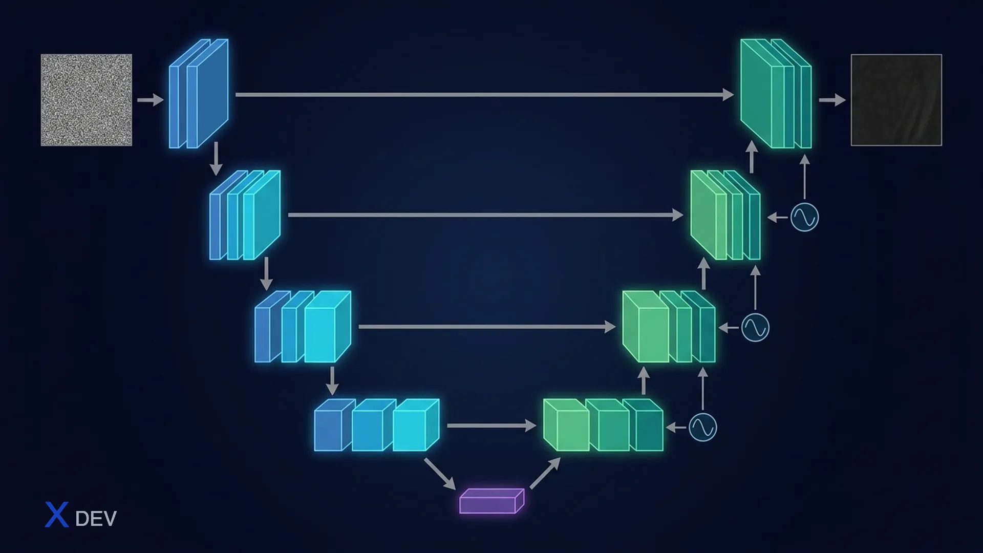
U-Net最初是為醫學影像中的影像分割而設計的(2015年,Ronneberger等人)。其特殊的架構——編碼器-解碼器加上跳躍連接——有助於在學習多層次抽象特徵的同時保留空間細節。這正是Diffusion Models所需要的。
考試提示:在評估中,你需要從零實作U-Net。理解每一層中張量維度是關鍵。NVIDIA DLI要求你撰寫可運行的程式碼,而不僅僅是理解理論。
2. U-Net架構:編碼器-解碼器與跳躍連接
2.1 架構概述
U-Net具有「U」形結構,包含3個主要部分:
- 編碼器(收縮路徑):降低空間解析度,增加通道數——學習高層次抽象特徵
- 瓶頸層:最小空間,最大通道數——捕捉全域上下文
- 解碼器(擴張路徑):增加空間解析度,減少通道數——恢復細節
- 跳躍連接:將編碼器特徵直接連接到對應的解碼器——保留精細細節
U-Net Architecture for Diffusion (input 64×64×1)
═══════════════════════════════════════════════

          ENCODER                              DECODER
     (Contracting Path)                   (Expanding Path)

  ┌─────────────────┐                 ┌─────────────────┐
  │  64 × 64 × 1    │   Input Image   │  64 × 64 × 1    │  Output (denoised)
  └────────┬────────┘                 └────────▲────────┘
           │                                    │
           ▼                                    │
  ┌─────────────────┐  skip connection  ┌─────────────────┐
  │  64 × 64 × 64   │ ───────────────► │  64 × 64 × 64   │  UpBlock + Concat
  │  Conv→GN→GELU   │   (concatenate)   │  Conv→GN→GELU   │
  └────────┬────────┘                 └────────▲────────┘
           │ Downsample                        │ Upsample
           ▼                                    │
  ┌─────────────────┐  skip connection  ┌─────────────────┐
  │  32 × 32 × 128  │ ───────────────► │  32 × 32 × 128  │  UpBlock + Concat
  │  Conv→GN→GELU   │   (concatenate)   │  Conv→GN→GELU   │
  └────────┬────────┘                 └────────▲────────┘
           │ Downsample                        │ Upsample
           ▼                                    │
  ┌─────────────────┐  skip connection  ┌─────────────────┐
  │  16 × 16 × 256  │ ───────────────► │  16 × 16 × 256  │  UpBlock + Concat
  │  Conv→GN→GELU   │   (concatenate)   │  Conv→GN→GELU   │
  └────────┬────────┘                 └────────▲────────┘
           │ Downsample                        │ Upsample
           ▼                                    │
  ┌──────────────────────────────────────────────┐
  │              8 × 8 × 512                      │
  │           BOTTLENECK                          │
  │     Conv → GN → GELU → Conv → GN             │
  │  (smallest spatial, largest channels)         │
  └───────────────────────────────────────────────┘

  + Timestep Embedding ──► injected into EVERY ResidualBlock via linear projection
2.2 編碼器路徑(收縮)
每個編碼器層級執行以下操作:
- 卷積:3×3卷積,padding=1(保持空間大小不變)
- Group Normalization:按組進行正規化,而非按批次
- GELU啟動函數:比ReLU更平滑的非線性函數
- 下取樣:將空間解析度降低2倍(可使用stride=2卷積或Rearrange Pooling)
在每個層級,通道數加倍且空間減半。例如:
| 層級 | 輸入形狀 | 輸出形狀 | 操作 |
|---|---|---|---|
| 0 | B × 1 × 64 × 64 | B × 64 × 64 × 64 | 初始卷積 |
| 1 | B × 64 × 64 × 64 | B × 128 × 32 × 32 | ResBlock → 下取樣 |
| 2 | B × 128 × 32 × 32 | B × 256 × 16 × 16 | ResBlock → 下取樣 |
| 3 | B × 256 × 16 × 16 | B × 512 × 8 × 8 | ResBlock → 下取樣 |
2.3 解碼器路徑(擴張)
與編碼器相反,解碼器增加空間解析度並減少通道數:
- 上取樣:將空間解析度增加2倍(通常使用
nn.Upsample或nn.ConvTranspose2d) - 與編碼器同一層級的跳躍連接進行串接
- 卷積 → GroupNorm → GELU:處理串接後的特徵
考試提示:串接跳躍連接時,通道數會暫時加倍。例如:上取樣輸出有256個通道 + 跳躍連接有256個通道 = 512個通道輸入到卷積層。這是常見的實作錯誤——請注意串接後卷積的
in_channels!
2.4 跳躍連接——為什麼重要?
沒有跳躍連接,解碼器必須僅從8×8瓶頸層「猜測」所有空間細節——幾乎不可能。跳躍連接能夠:
- 梯度流動:梯度直接從損失函數流回深層編碼器——更容易訓練
- 細節保留:高層編碼器保留了邊緣和紋理——解碼器重複利用而非重新學習
- 多尺度特徵:解碼器同時接收高層次(來自瓶頸層)和低層次(來自跳躍連接)的特徵
3. 關鍵組件:GroupNorm、GELU、Rearrange Pooling
3.1 Group Normalization
在Diffusion Models中,批次大小通常非常小(4-8),因為每張圖像消耗大量GPU記憶體。Batch Normalization在小批次下表現不佳,因為基於批次計算的統計量(均值、變異數)不穩定。
Group Normalization透過將通道分成組並在每組內、每個樣本獨立地進行正規化來解決這個問題——與批次大小無關。
Group Normalization vs Batch Normalization
══════════════════════════════════════════

Batch Normalization:              Group Normalization:
  normalize across N (batch)        normalize within groups of C

  ┌───┬───┬───┬───┐               ┌───┬───┬───┬───┐
  │ N │   │   │   │               │   │   │   │   │  N (batch)
  ├───┼───┼───┼───┤               ├───┼───┼───┼───┤
  │   │   │   │   │  C            │ G1│ G1│ G2│ G2│  C (channels)
  ├───┼───┼───┼───┤  (channels)   ├───┼───┼───┼───┤  split into groups
  │   │   │   │   │               │ G1│ G1│ G2│ G2│
  ├───┼───┼───┼───┤               ├───┼───┼───┼───┤
  │   │   │   │   │  H×W          │   │   │   │   │  H×W
  └───┴───┴───┴───┘               └───┴───┴───┴───┘
     ▲                                 ▲
     normalize column (across N)       normalize block (within group)
     ⚠ small batch → unstable          ✓ independent of batch size
import torch.nn as nn

# GroupNorm:將64個通道分成8組(每組8個通道)
norm = nn.GroupNorm(num_groups=8, num_channels=64)

# 輸入形狀為(B, 64, 32, 32)時:
# - 將64個通道分成8組,每組8個通道
# - 對每個樣本、每組計算均值和變異數,計算範圍為(8, 32, 32) = 8192個元素
# - 對每個樣本、每組獨立正規化

x = torch.randn(4, 64, 32, 32)
out = norm(x)  # 形狀:(4, 64, 32, 32)——形狀不變
| 特性 | BatchNorm | GroupNorm | LayerNorm | InstanceNorm |
|---|---|---|---|---|
| 正規化維度 | 批次(N) | 通道組 | 所有通道 | 每個通道 |
| 依賴批次大小 | 是 ⚠ | 否 ✓ | 否 ✓ | 否 ✓ |
| 小批次效能 | 差 | 好 | 尚可 | 尚可 |
| 適用場景 | 分類 | Diffusion、偵測 | Transformers(NLP) | 風格轉換 |
| PyTorch API | nn.BatchNorm2d(C) | nn.GroupNorm(G, C) | nn.LayerNorm(shape) | nn.InstanceNorm2d(C) |
3.2 GELU啟動函數
GELU(Gaussian Error Linear Unit)是現代模型(Transformers、Diffusion Models)中的標準啟動函數。與「硬」ReLU(將負值截斷為0)不同,GELU是平滑的,允許部分負值「洩漏」通過。
公式:GELU(x) = x · Φ(x),其中Φ(x)是標準常態分佈的累積分佈函數。
Activation Functions Comparison
═══════════════════════════════

 Output                              Output
   │     ReLU                          │     GELU
   │      ╱                            │      ╱
   │     ╱                             │    ╱
   │    ╱                              │  ╱
───┼───╱────── Input            ───┼──╱─────── Input
   │  ╱                              ╱│
   │ ╱                              ╱ │
   │╱  (hard cutoff at 0)         ╱  │  (smooth curve, allows
   │                             ╱    │   small negative values)

 ReLU(x) = max(0, x)           GELU(x) = x · Φ(x)
 ⚠ Dead neurons problem         ✓ Smoother gradient flow
 ⚠ Not differentiable at 0      ✓ Better for deep networks
import torch.nn as nn

# 方法1:使用模組
activation = nn.GELU()
out = activation(x)

# 方法2:使用函數式介面
import torch.nn.functional as F
out = F.gelu(x)

# 方法3:近似計算(更快,DLI課程中使用)
activation = nn.GELU(approximate='tanh')
3.3 Rearrange Pooling(空間轉通道)
Rearrange Pooling是一種取代MaxPool/AvgPool的下取樣技術。與丟棄資訊(MaxPool取最大值,AvgPool取平均值)不同,Rearrange將空間維度「摺疊」到通道維度——保留所有資訊。
Rearrange Pooling: (B, C, 2H, 2W) → (B, 4C, H, W)
════════════════════════════════════════════════════

Input: (B, C, 4, 4)                   Output: (B, 4C, 2, 2)

Channel c:                             4 channels (each is 1 "position"):
┌───┬───┬───┬───┐                     Channel c_0:    Channel c_1:
│ a │ b │ e │ f │                     ┌───┬───┐       ┌───┬───┐
├───┼───┼───┼───┤                     │ a │ e │       │ b │ f │
│ c │ d │ g │ h │      ────►         ├───┼───┤       ├───┼───┤
├───┼───┼───┼───┤   Rearrange        │ i │ m │       │ j │ n │
│ i │ j │ m │ n │                     └───┴───┘       └───┴───┘
├───┼───┼───┼───┤
│ k │ l │ o │ p │                     Channel c_2:    Channel c_3:
└───┴───┴───┴───┘                     ┌───┬───┐       ┌───┬───┐
                                       │ c │ g │       │ d │ h │
Spatial: 4×4, Channels: C             ├───┼───┤       ├───┼───┤
                                       │ k │ o │       │ l │ p │
                                       └───┴───┘       └───┴───┘

                                       Spatial: 2×2, Channels: 4C
                                       ✓ NO information loss!
from einops import rearrange

def rearrange_downsample(x):
    """Downsample by rearranging spatial dims into channels.
    (B, C, H, W) -> (B, 4C, H/2, W/2)
    """
    return rearrange(x, 'b c (h p1) (w p2) -> b (c p1 p2) h w', p1=2, p2=2)

# Example:
x = torch.randn(2, 64, 32, 32)
out = rearrange_downsample(x)
print(out.shape)  # torch.Size([2, 256, 16, 16])

# Without einops, using pure PyTorch:
def rearrange_downsample_pure(x):
    B, C, H, W = x.shape
    x = x.reshape(B, C, H // 2, 2, W // 2, 2)
    x = x.permute(0, 1, 3, 5, 2, 4)  # (B, C, 2, 2, H/2, W/2)
    x = x.reshape(B, C * 4, H // 2, W // 2)
    return x
| 下取樣方法 | 資訊損失 | 通道變化 | 在Diffusion中的使用 |
|---|---|---|---|
| MaxPool2d | 高(僅保留最大值) | 不變 | 很少使用 |
| AvgPool2d | 中(取平均值) | 不變 | 很少使用 |
| Stride-2卷積 | 可學習(可訓練) | 可配置 | 常見 |
| Rearrange Pooling | 無 ✓ | ×4 | NVIDIA DLI課程 ✓ |
考試提示:NVIDIA DLI使用Rearrange Pooling而非MaxPool。在評估中,你可能需要使用
einops.rearrange或純PyTorch(reshape+permute)來實作此函數。記住,當空間在每個維度上減少2倍時,通道數會增加4倍。
4. 用於時間步的正弦位置嵌入
4.1 為什麼需要時間步嵌入?
U-Net需要知道自己處於擴散過程的哪個時間步,才能適當地進行去噪:
- 大時間步(t接近T):圖像幾乎是純雜訊→模型需要恢復整體結構
- 小時間步(t接近0):圖像幾乎是乾淨的→模型只需要微調小細節
我們將整數時間步t轉換為長度為embed_dim的連續嵌入向量,注入到U-Net的每一層中。
4.2 正弦嵌入公式
與Transformer中的位置編碼(「Attention Is All You Need」)相同:
PE(t, 2i)   = sin(t / 10000^(2i/d))
PE(t, 2i+1) = cos(t / 10000^(2i/d))

Where:
  t = timestep (integer: 0, 1, 2, ..., T)
  d = embedding dimension (e.g., 128)
  i = index in embedding vector (0, 1, 2, ..., d/2 - 1)

Example with d=8:
  PE(t) = [sin(t/1), cos(t/1), sin(t/100), cos(t/100),
           sin(t/10000), cos(t/10000), sin(t/1000000), cos(t/1000000)]

  → Low frequency terms (end): change slowly → encode "big picture" timestep
  → High frequency terms (start): change rapidly → encode fine timestep differences
4.3 實作TimestepEmbedding
import torch
import torch.nn as nn
import math

class SinusoidalPositionEmbedding(nn.Module):
    """Convert integer timestep to sinusoidal embedding vector."""

    def __init__(self, embed_dim):
        super().__init__()
        self.embed_dim = embed_dim

    def forward(self, timesteps):
        """
        Args:
            timesteps: (B,) — integer timesteps
        Returns:
            embeddings: (B, embed_dim) — sinusoidal embeddings
        """
        device = timesteps.device
        half_dim = self.embed_dim // 2

        # Compute frequencies: 1/10000^(2i/d) for i = 0, 1, ..., d/2-1
        exponent = torch.arange(half_dim, device=device).float() / half_dim
        freqs = torch.exp(-math.log(10000.0) * exponent)  # shape: (d/2,)

        # Multiply timestep by frequencies: (B, 1) * (1, d/2) = (B, d/2)
        args = timesteps[:, None].float() * freqs[None, :]

        # Concat sin and cos: (B, d/2) cat (B, d/2) = (B, d)
        embeddings = torch.cat([torch.sin(args), torch.cos(args)], dim=-1)

        return embeddings  # shape: (B, embed_dim)


class TimestepMLPEmbedding(nn.Module):
    """Sinusoidal embedding + MLP projection (used in DLI course)."""

    def __init__(self, embed_dim, hidden_dim=None):
        super().__init__()
        if hidden_dim is None:
            hidden_dim = embed_dim * 4

        self.sinusoidal = SinusoidalPositionEmbedding(embed_dim)
        self.mlp = nn.Sequential(
            nn.Linear(embed_dim, hidden_dim),
            nn.GELU(),
            nn.Linear(hidden_dim, hidden_dim),
        )

    def forward(self, timesteps):
        """
        Args:
            timesteps: (B,) — integer timesteps
        Returns:
            (B, hidden_dim) — projected timestep embeddings
        """
        x = self.sinusoidal(timesteps)  # (B, embed_dim)
        x = self.mlp(x)                 # (B, hidden_dim)
        return x
4.4 將時間步注入U-Net
時間步嵌入透過以下方式注入到每個ResidualBlock中:
- 將時間步嵌入投影到與特徵圖通道數匹配(使用
nn.Linear) - 重塑為
(B, C, 1, 1)以進行廣播 - 加到第一個GroupNorm之後的特徵圖上
Timestep Injection Flow
═══════════════════════

timestep t ──► SinusoidalEmbed ──► MLP ──► t_emb (B, hidden_dim)
                                              │
                                    Linear(hidden_dim, C)
                                              │
                                         (B, C, 1, 1)   ← reshape for broadcasting
                                              │
Feature Map: ─── Conv ─── GroupNorm ────── (+) ────── GELU ─── Conv ─── ...
                                          add here
考試提示:時間步嵌入是相加的,而非串接到特徵圖上。注入發生在每個ResidualBlock中GroupNorm之後、GELU之前。這是DLI課程中的固定模式。
5. 從零建構U-Net——逐步實作
5.1 ResidualBlock
這是最基礎的構建單元。每個ResidualBlock由2個卷積層 + GroupNorm + GELU組成,加上殘差連接和時間步注入。
class ResidualBlock(nn.Module):
    """Residual block with timestep embedding injection.

    Flow: x → Conv1 → GN1 → (+t_emb) → GELU → Conv2 → GN2 → GELU → (+residual) → out
    """

    def __init__(self, in_channels, out_channels, time_emb_dim):
        super().__init__()

        # First conv layer
        self.conv1 = nn.Conv2d(in_channels, out_channels, kernel_size=3, padding=1)
        self.norm1 = nn.GroupNorm(num_groups=8, num_channels=out_channels)

        # Second conv layer
        self.conv2 = nn.Conv2d(out_channels, out_channels, kernel_size=3, padding=1)
        self.norm2 = nn.GroupNorm(num_groups=8, num_channels=out_channels)

        # Activation
        self.act = nn.GELU()

        # Timestep embedding projection: project to out_channels
        self.time_mlp = nn.Sequential(
            nn.GELU(),
            nn.Linear(time_emb_dim, out_channels),
        )

        # Residual connection: if in_channels != out_channels, need 1x1 conv
        if in_channels != out_channels:
            self.residual_conv = nn.Conv2d(in_channels, out_channels, kernel_size=1)
        else:
            self.residual_conv = nn.Identity()

    def forward(self, x, t_emb):
        """
        Args:
            x: (B, in_channels, H, W) — input feature map
            t_emb: (B, time_emb_dim) — timestep embedding
        Returns:
            (B, out_channels, H, W)
        """
        residual = self.residual_conv(x)   # (B, out_channels, H, W)

        # First layer
        h = self.conv1(x)                   # (B, out_channels, H, W)
        h = self.norm1(h)                   # normalize

        # Inject timestep embedding
        t = self.time_mlp(t_emb)            # (B, out_channels)
        t = t[:, :, None, None]             # (B, out_channels, 1, 1) broadcast
        h = h + t                           # add timestep info

        h = self.act(h)                     # GELU activation

        # Second layer
        h = self.conv2(h)                   # (B, out_channels, H, W)
        h = self.norm2(h)                   # normalize
        h = self.act(h)                     # GELU activation

        return h + residual                  # residual connection
5.2 DownBlock(編碼器層級)
class DownBlock(nn.Module):
    """Encoder block: ResidualBlock + Rearrange Downsample."""

    def __init__(self, in_channels, out_channels, time_emb_dim):
        super().__init__()
        self.res_block = ResidualBlock(in_channels, out_channels, time_emb_dim)

    def downsample(self, x):
        """Rearrange pooling: (B, C, H, W) -> (B, 4C, H/2, W/2)"""
        B, C, H, W = x.shape
        x = x.reshape(B, C, H // 2, 2, W // 2, 2)
        x = x.permute(0, 1, 3, 5, 2, 4).reshape(B, C * 4, H // 2, W // 2)
        return x

    def forward(self, x, t_emb):
        """
        Args:
            x: (B, in_channels, H, W)
            t_emb: (B, time_emb_dim)
        Returns:
            skip: (B, out_channels, H, W) — for skip connection
            down: (B, out_channels*4, H/2, W/2) — downsampled for next level
        """
        skip = self.res_block(x, t_emb)    # (B, out_channels, H, W)
        down = self.downsample(skip)         # (B, out_channels*4, H/2, W/2)
        return skip, down
5.3 UpBlock(解碼器層級)
class UpBlock(nn.Module):
    """Decoder block: Upsample + Concat skip + ResidualBlock."""

    def __init__(self, in_channels, skip_channels, out_channels, time_emb_dim):
        super().__init__()
        # in_channels = channels from below level after upsample
        # After concat with skip: in_channels + skip_channels
        self.res_block = ResidualBlock(
            in_channels + skip_channels, out_channels, time_emb_dim
        )
        self.upsample = nn.Upsample(scale_factor=2, mode='nearest')

    def forward(self, x, skip, t_emb):
        """
        Args:
            x: (B, in_channels, H, W) — from below level
            skip: (B, skip_channels, 2H, 2W) — skip connection from encoder
            t_emb: (B, time_emb_dim)
        Returns:
            (B, out_channels, 2H, 2W)
        """
        x = self.upsample(x)               # (B, in_channels, 2H, 2W)
        x = torch.cat([x, skip], dim=1)     # (B, in_channels+skip_channels, 2H, 2W)
        x = self.res_block(x, t_emb)        # (B, out_channels, 2H, 2W)
        return x
5.4 完整U-Net組裝
class UNet(nn.Module):
    """Complete U-Net for diffusion denoising.

    Architecture: 64×64×1 → encoder (3 levels) → bottleneck → decoder (3 levels) → 64×64×1
    Channel progression: 1 → 64 → 128 → 256 → 512 (bottleneck) → 256 → 128 → 64 → 1
    """

    def __init__(self, in_channels=1, base_channels=64, time_emb_dim=128):
        super().__init__()

        # Timestep embedding
        self.time_embed = TimestepMLPEmbedding(
            embed_dim=time_emb_dim,
            hidden_dim=time_emb_dim * 4
        )
        t_dim = time_emb_dim * 4  # output dim of MLP

        # Initial convolution: 1 → 64
        self.init_conv = nn.Conv2d(in_channels, base_channels, kernel_size=3, padding=1)

        # Encoder path
        # Level 1: 64ch, 64×64 → Rearrange → 256ch, 32×32
        self.down1 = DownBlock(base_channels, base_channels, t_dim)        # 64 → 64 (skip), 256 (down)

        # Level 2: 256ch, 32×32 → Rearrange → 512ch, 16×16
        # Need 1x1 conv before because Rearrange creates 4× channels
        self.down1_proj = nn.Conv2d(base_channels * 4, base_channels * 2, kernel_size=1)
        self.down2 = DownBlock(base_channels * 2, base_channels * 2, t_dim) # 128 → 128 (skip), 512 (down)

        # Level 3: 512ch, 16×16 → Rearrange → 1024ch, 8×8
        self.down2_proj = nn.Conv2d(base_channels * 8, base_channels * 4, kernel_size=1)
        self.down3 = DownBlock(base_channels * 4, base_channels * 4, t_dim) # 256 → 256 (skip), 1024 (down)

        # Bottleneck: 1024ch, 8×8 → 512ch, 8×8
        self.down3_proj = nn.Conv2d(base_channels * 16, base_channels * 8, kernel_size=1)
        self.bottleneck = ResidualBlock(base_channels * 8, base_channels * 8, t_dim)  # 512 → 512

        # Decoder path
        # Level 3: upsample 512 to 16×16, concat skip(256) → 768 → 256
        self.up3 = UpBlock(base_channels * 8, base_channels * 4, base_channels * 4, t_dim)

        # Level 2: upsample 256 to 32×32, concat skip(128) → 384 → 128
        self.up2 = UpBlock(base_channels * 4, base_channels * 2, base_channels * 2, t_dim)

        # Level 1: upsample 128 to 64×64, concat skip(64) → 192 → 64
        self.up1 = UpBlock(base_channels * 2, base_channels, base_channels, t_dim)

        # Final output: 64 → 1
        self.final_conv = nn.Sequential(
            nn.GroupNorm(8, base_channels),
            nn.GELU(),
            nn.Conv2d(base_channels, in_channels, kernel_size=1),
        )

    def forward(self, x, timesteps):
        """
        Args:
            x: (B, 1, 64, 64) — noisy image
            timesteps: (B,) — integer timesteps
        Returns:
            (B, 1, 64, 64) — predicted clean image (or noise)
        """
        # Timestep embedding
        t_emb = self.time_embed(timesteps)    # (B, t_dim)

        # Initial conv
        x = self.init_conv(x)                 # (B, 64, 64, 64)

        # Encoder
        skip1, x = self.down1(x, t_emb)       # skip1: (B,64,64,64), x: (B,256,32,32)
        x = self.down1_proj(x)                 # (B, 128, 32, 32)

        skip2, x = self.down2(x, t_emb)       # skip2: (B,128,32,32), x: (B,512,16,16)
        x = self.down2_proj(x)                 # (B, 256, 16, 16)

        skip3, x = self.down3(x, t_emb)       # skip3: (B,256,16,16), x: (B,1024,8,8)
        x = self.down3_proj(x)                 # (B, 512, 8, 8)

        # Bottleneck
        x = self.bottleneck(x, t_emb)         # (B, 512, 8, 8)

        # Decoder
        x = self.up3(x, skip3, t_emb)         # (B, 256, 16, 16)
        x = self.up2(x, skip2, t_emb)         # (B, 128, 32, 32)
        x = self.up1(x, skip1, t_emb)         # (B, 64, 64, 64)

        # Final output
        x = self.final_conv(x)                 # (B, 1, 64, 64)
        return x
驗證張量形狀:
# Verify shapes
model = UNet(in_channels=1, base_channels=64, time_emb_dim=128)
x = torch.randn(2, 1, 64, 64)
t = torch.randint(0, 1000, (2,))
out = model(x, t)
print(f"Input:  {x.shape}")    # torch.Size([2, 1, 64, 64])
print(f"Output: {out.shape}")  # torch.Size([2, 1, 64, 64])
print(f"Params: {sum(p.numel() for p in model.parameters()):,}")
Tensor Shape Flow through U-Net (base_channels=64)
═══════════════════════════════════════════════

Layer                    Shape                  Notes
──────────────────────────────────────────────────────────
Input                    (B, 1, 64, 64)
init_conv                (B, 64, 64, 64)        Conv2d(1, 64)

down1 ResBlock           (B, 64, 64, 64)        skip1 ─────────────────┐
down1 Rearrange          (B, 256, 32, 32)       4× channels            │
down1_proj               (B, 128, 32, 32)       1×1 conv reduce        │
                                                                        │
down2 ResBlock           (B, 128, 32, 32)       skip2 ──────────┐      │
down2 Rearrange          (B, 512, 16, 16)       4× channels     │      │
down2_proj               (B, 256, 16, 16)       1×1 conv reduce │      │
                                                                 │      │
down3 ResBlock           (B, 256, 16, 16)       skip3 ───┐      │      │
down3 Rearrange          (B, 1024, 8, 8)        4× ch    │      │      │
down3_proj               (B, 512, 8, 8)         reduce   │      │      │
                                                          │      │      │
bottleneck               (B, 512, 8, 8)                   │      │      │
                                                          │      │      │
up3 Upsample             (B, 512, 16, 16)                │      │      │
up3 Concat skip3         (B, 768, 16, 16) ◄──────────────┘      │      │
up3 ResBlock             (B, 256, 16, 16)                        │      │
                                                                  │      │
up2 Upsample             (B, 256, 32, 32)                        │      │
up2 Concat skip2         (B, 384, 32, 32) ◄─────────────────────┘      │
up2 ResBlock             (B, 128, 32, 32)                               │
                                                                         │
up1 Upsample             (B, 128, 64, 64)                               │
up1 Concat skip1         (B, 192, 64, 64) ◄────────────────────────────┘
up1 ResBlock             (B, 64, 64, 64)

final_conv               (B, 1, 64, 64)         Output = denoised image
考試提示:在評估中,你需要精確計算張量形狀。記住規則:Rearrange → 通道×4,空間÷2。串接跳躍連接後,通道數 = 上取樣的通道 + 跳躍連接的通道。在寫程式碼之前先在草稿紙上寫下這些!
6. 訓練去噪模型
6.1 簡單去噪任務
在學習完整的擴散過程(多個時間步)之前,我們先從一個簡單任務開始:
向圖像添加高斯雜訊→訓練U-Net恢復原始圖像
Simple Denoising Task
═════════════════════

Original Image        Add Noise                Noisy Image        U-Net         Denoised Output
   ┌──────┐          ┌──────┐                  ┌──────┐         ┌─────┐         ┌──────┐
   │ 🖼️   │    +     │ ░░░░ │  noise_level     │ ░🖼️░ │  ────► │U-Net│  ────►  │ 🖼️   │
   │      │          │ ░░░░ │  * N(0,1)        │ ░░░░ │         │     │         │      │
   └──────┘          └──────┘                  └──────┘         └─────┘         └──────┘
      x₀               ε                      x_noisy          predict          x̂₀
                                            = x₀ + σ·ε           x₀

Loss = MSE(x̂₀, x₀) = ‖U-Net(x_noisy, t) - x₀‖²
6.2 訓練迴圈
import torch
import torch.nn as nn
import torch.optim as optim
from torch.utils.data import DataLoader
from torchvision import datasets, transforms

# 超參數
BATCH_SIZE = 32
LEARNING_RATE = 1e-4
EPOCHS = 50
NOISE_LEVEL = 0.5  # σ:控制添加雜訊的量
DEVICE = torch.device('cuda' if torch.cuda.is_available() else 'cpu')

# 資料集:MNIST(灰階28×28→調整至64×64)
transform = transforms.Compose([
    transforms.Resize((64, 64)),
    transforms.ToTensor(),           # [0, 1]
    transforms.Normalize([0.5], [0.5])  # [-1, 1]
])
dataset = datasets.MNIST(root='./data', train=True, transform=transform, download=True)
dataloader = DataLoader(dataset, batch_size=BATCH_SIZE, shuffle=True)

# 模型、優化器、損失函數
model = UNet(in_channels=1, base_channels=64, time_emb_dim=128).to(DEVICE)
optimizer = optim.Adam(model.parameters(), lr=LEARNING_RATE)
loss_fn = nn.MSELoss()

# 訓練迴圈
for epoch in range(EPOCHS):
    total_loss = 0
    for batch_idx, (images, _) in enumerate(dataloader):
        images = images.to(DEVICE)                    # (B, 1, 64, 64)

        # 隨機時間步(每個樣本獲得不同的時間步)
        timesteps = torch.randint(0, 1000, (images.shape[0],), device=DEVICE)

        # 根據時間步縮放雜訊等級(簡單方式:線性縮放)
        noise_scales = (timesteps.float() / 1000.0 * NOISE_LEVEL)  # (B,)
        noise_scales = noise_scales[:, None, None, None]             # (B,1,1,1)

        # 添加雜訊
        noise = torch.randn_like(images)                             # (B, 1, 64, 64)
        noisy_images = images + noise_scales * noise                 # (B, 1, 64, 64)

        # 前向傳播:預測乾淨圖像
        predicted_clean = model(noisy_images, timesteps)             # (B, 1, 64, 64)

        # 損失:預測乾淨圖像與實際乾淨圖像之間的MSE
        loss = loss_fn(predicted_clean, images)

        # 反向傳播
        optimizer.zero_grad()
        loss.backward()
        optimizer.step()

        total_loss += loss.item()

    avg_loss = total_loss / len(dataloader)
    print(f"Epoch [{epoch+1}/{EPOCHS}], Loss: {avg_loss:.6f}")
6.3 視覺化結果
import matplotlib.pyplot as plt

@torch.no_grad()
def visualize_denoising(model, dataloader, noise_level=0.5, num_images=5):
    """Display: Original → Noisy → Denoised."""
    model.eval()
    images, _ = next(iter(dataloader))
    images = images[:num_images].to(DEVICE)

    # Add noise
    timesteps = torch.full((num_images,), 500, device=DEVICE)
    noise = torch.randn_like(images) * noise_level
    noisy = images + noise

    # Denoise
    denoised = model(noisy, timesteps)

    # Plot
    fig, axes = plt.subplots(3, num_images, figsize=(num_images * 3, 9))
    titles = ['Original', 'Noisy', 'Denoised']

    for i in range(num_images):
        for j, (img, title) in enumerate(zip(
            [images[i], noisy[i], denoised[i]], titles
        )):
            ax = axes[j][i]
            # Denormalize: [-1,1] → [0,1]
            img_np = (img.cpu().squeeze() * 0.5 + 0.5).clamp(0, 1).numpy()
            ax.imshow(img_np, cmap='gray')
            ax.set_title(title if i == 0 else '')
            ax.axis('off')

    plt.tight_layout()
    plt.savefig('denoising_results.png', dpi=150)
    plt.show()

visualize_denoising(model, dataloader)
考試提示:在評估中,你可能需要完成訓練迴圈。記住3個重要步驟:(1)向乾淨圖像添加雜訊,(2)將帶雜訊圖像+時間步通過U-Net前向傳播,(3)計算預測值與原始值之間的MSE損失。不要忘記將時間步傳遞給模型!
7. 速查表——U-Net與去噪
| 概念 | 關鍵細節 | 程式碼/公式 |
|---|---|---|
| U-Net結構 | 編碼器→瓶頸層→解碼器 + 跳躍連接 | U形,跳躍連接=串接 |
| GroupNorm | 按組正規化,與批次大小無關 | nn.GroupNorm(8, channels) |
| GELU | 平滑啟動函數,x·Φ(x) | nn.GELU() |
| Rearrange Pooling | (B,C,2H,2W)→(B,4C,H,W),無損 | rearrange(x, 'b c (h p1) (w p2) → b (c p1 p2) h w', p1=2, p2=2) |
| 正弦嵌入 | 不同頻率的sin/cos | sin(t/10000^(2i/d))、cos(t/10000^(2i/d)) |
| 時間步注入 | 在GroupNorm之後加到特徵圖上 | h = h + t_emb[:,:,None,None] |
| ResidualBlock | Conv→GN→(+t)→GELU→Conv→GN→GELU + 跳躍 | 2個卷積層 + 殘差 + 時間步 |
| 去噪損失 | 預測乾淨圖像與實際乾淨圖像之間的MSE | MSE(model(x_noisy, t), x_clean) |
| 跳躍連接的作用 | 保留空間細節,改善梯度流動 | torch.cat([upsample, skip], dim=1) |
| 串接後的通道數 | 上取樣的通道 + 跳躍連接的通道 | 必須與下一層卷積的in_channels匹配 |
8. 練習題
以下題目模擬NVIDIA DLI程式碼評估。請先嘗試自己寫程式碼,再查看答案!
Q1:實作帶有時間步注入的ResidualBlock
完成下方ResidualBlock的forward方法。該區塊應該使用GroupNorm和GELU進行兩層卷積,在第一次正規化後注入時間步嵌入,並加上殘差連接。
class ResidualBlock(nn.Module):
    def __init__(self, in_ch, out_ch, t_dim):
        super().__init__()
        self.conv1 = nn.Conv2d(in_ch, out_ch, 3, padding=1)
        self.norm1 = nn.GroupNorm(8, out_ch)
        self.conv2 = nn.Conv2d(out_ch, out_ch, 3, padding=1)
        self.norm2 = nn.GroupNorm(8, out_ch)
        self.act = nn.GELU()
        self.time_proj = nn.Linear(t_dim, out_ch)
        self.res_conv = nn.Conv2d(in_ch, out_ch, 1) if in_ch != out_ch else nn.Identity()

    def forward(self, x, t_emb):
        # TODO: implement this method
        pass
顯示答案 Q1
def forward(self, x, t_emb):
    residual = self.res_conv(x)

    h = self.conv1(x)
    h = self.norm1(h)

    # Inject timestep: project t_emb to out_ch, reshape for broadcasting, add
    t = self.time_proj(t_emb)          # (B, out_ch)
    t = t[:, :, None, None]            # (B, out_ch, 1, 1)
    h = h + t

    h = self.act(h)

    h = self.conv2(h)
    h = self.norm2(h)
    h = self.act(h)

    return h + residual
解說:關鍵要點——(1)時間步是相加的,不是串接的,(2)重塑為(B, C, 1, 1)使其能在H×W上廣播,(3)注入發生在norm1之後、GELU之前,(4)當通道維度不匹配時,殘差使用1×1卷積。
Q2:如果移除U-Net的跳躍連接會發生什麼?
考慮以下修改過的U-Net,解碼器中不使用跳躍連接:
# Original (with skip connections):
x = self.upsample(x)
x = torch.cat([x, skip], dim=1)  # concat skip
x = self.res_block(x, t_emb)

# Modified (WITHOUT skip connections):
x = self.upsample(x)
# skip connection removed!
x = self.res_block(x, t_emb)
去噪輸出會發生什麼?選擇所有適用的選項:
- A) 輸出會模糊,丟失精細細節
- B) 模型因形狀不匹配而無法編譯
- C) 訓練損失會顯著增加
- D) 無論輸入為何,模型產生相同的輸出
顯示答案 Q2
A和C是正確答案。
解說:(A)沒有跳躍連接,解碼器只能從瓶頸層資訊(512通道的8×8)重建64×64的細節——精細紋理和邊緣會丟失,導致模糊的輸出。(B)如果適當調整res_block的in_channels則不會有形狀不匹配——若配置正確不會有形狀不匹配。(C)正確——模型可用來重建的資訊更少,因此預測與乾淨圖像之間的MSE損失會更高。(D)這只在極端情況下才會發生,例如完全的資訊瓶頸。模型仍然可以從瓶頸層特徵捕捉大致結構。
Q3:計算U-Net每一層級的輸出形狀
給定以下U-Net配置,填入缺失的張量形狀:
# Config: in_channels=1, base_channels=32, image_size=32×32
# Using Rearrange Pooling for downsampling

x = input                  # Shape: (B, 1, 32, 32)
x = init_conv(x)           # Shape: (B, 32, 32, 32)

# Encoder Level 1
skip1, x = down1(x)        # skip1: (B, 32, 32, 32),  x after rearrange: ???
x = proj1(x)               # Shape: ???

# Encoder Level 2
skip2, x = down2(x)        # skip2: ???,  x after rearrange: ???
x = proj2(x)               # Shape: ???

# Bottleneck
x = bottleneck(x)          # Shape: ???

# Decoder Level 2
x = upsample(x)            # Shape: ???
x = cat(x, skip2)          # Shape: ???
x = res_block(x)           # Shape: ???

# Decoder Level 1
x = upsample(x)            # Shape: ???
x = cat(x, skip1)          # Shape: ???
x = res_block(x)           # Shape: ???

x = final_conv(x)          # Shape: (B, 1, 32, 32)
顯示答案 Q3
x = input                  # (B, 1, 32, 32)
x = init_conv(x)           # (B, 32, 32, 32)

# Encoder Level 1
skip1 = res1(x)            # skip1: (B, 32, 32, 32)
x = rearrange(skip1)       # (B, 128, 16, 16)      ← 32×4=128, 32/2=16
x = proj1(x)               # (B, 64, 16, 16)       ← 1×1 conv reduce

# Encoder Level 2
skip2 = res2(x)            # skip2: (B, 64, 16, 16)
x = rearrange(skip2)       # (B, 256, 8, 8)         ← 64×4=256, 16/2=8
x = proj2(x)               # (B, 128, 8, 8)         ← 1×1 conv reduce

# Bottleneck
x = bottleneck(x)          # (B, 128, 8, 8)

# Decoder Level 2
x = upsample(x)            # (B, 128, 16, 16)       ← spatial ×2
x = cat(x, skip2)          # (B, 192, 16, 16)       ← 128+64=192
x = res_block(x)           # (B, 64, 16, 16)        ← project down

# Decoder Level 1
x = upsample(x)            # (B, 64, 32, 32)        ← spatial ×2
x = cat(x, skip1)          # (B, 96, 32, 32)        ← 64+32=96
x = res_block(x)           # (B, 32, 32, 32)        ← project down

x = final_conv(x)          # (B, 1, 32, 32)
解說:關鍵模式——Rearrange Pooling將通道數乘以4,空間維度減半。串接跳躍連接後,通道數 = 上取樣通道數 + 跳躍連接通道數。仔細追蹤這些數值以正確設定每層的in_channels。
Q4:實作SinusoidalPositionEmbedding類別
實作將整數時間步轉換為正弦嵌入的forward方法:
class SinusoidalPositionEmbedding(nn.Module):
    def __init__(self, embed_dim):
        super().__init__()
        self.embed_dim = embed_dim  # must be even

    def forward(self, timesteps):
        """
        Args:
            timesteps: (B,) — integer timesteps
        Returns:
            (B, embed_dim) — sinusoidal embeddings
        """
        # TODO: implement using formula:
        # PE(t, 2i) = sin(t / 10000^(2i/d))
        # PE(t, 2i+1) = cos(t / 10000^(2i/d))
        pass
顯示答案 Q4
import math

def forward(self, timesteps):
    device = timesteps.device
    half_dim = self.embed_dim // 2

    # Step 1: Compute frequency terms
    # exp(-log(10000) * i/(d/2)) = 1/10000^(i/(d/2)) for i in [0, d/2)
    freqs = torch.exp(
        -math.log(10000.0) * torch.arange(half_dim, device=device).float() / half_dim
    )

    # Step 2: Outer product of timesteps and frequencies
    # (B, 1) * (1, d/2) → (B, d/2)
    args = timesteps[:, None].float() * freqs[None, :]

    # Step 3: Apply sin and cos, concatenate
    embeddings = torch.cat([torch.sin(args), torch.cos(args)], dim=-1)
    # Result shape: (B, embed_dim)

    return embeddings
解說:三個關鍵步驟——(1)使用exp(-log(10000) * i/half_dim)計算頻率項,這等同於1/10000^(2i/d),(2)透過廣播將每個時間步乘以所有頻率,(3)對前半部分應用sin,後半部分應用cos,然後串接。math.log(10000.0)的公式在數值上比直接計算10000**(2i/d)更穩定。
Q5:除錯U-Net——輸出始終是訓練集的平均值
一位學生實作了用於去噪的U-Net,但無論輸入為何,輸出始終看起來像MNIST數字的模糊平均值。檢查以下程式碼並找出錯誤:
class BuggyUpBlock(nn.Module):
    def __init__(self, in_channels, out_channels, time_emb_dim):
        super().__init__()
        self.upsample = nn.Upsample(scale_factor=2, mode='nearest')
        # BUG: Notice in_channels here — where is the skip connection?
        self.res_block = ResidualBlock(in_channels, out_channels, time_emb_dim)

    def forward(self, x, skip, t_emb):
        x = self.upsample(x)
        # BUG: skip connection is received but never used!
        x = self.res_block(x, t_emb)
        return x


class BuggyUNet(nn.Module):
    def __init__(self):
        super().__init__()
        # ... encoder and bottleneck (correct) ...

        # Decoder — uses BuggyUpBlock
        self.up3 = BuggyUpBlock(512, 256, t_dim)  # skip not concatenated
        self.up2 = BuggyUpBlock(256, 128, t_dim)   # skip not concatenated
        self.up1 = BuggyUpBlock(128, 64, t_dim)    # skip not concatenated
錯誤是什麼?如何修復?
顯示答案 Q5
錯誤:skip張量被傳遞給forward()但從未與x串接。解碼器只看到瓶頸層特徵(重度壓縮的8×8),無法重建空間細節→輸出收斂到資料集平均值。
class FixedUpBlock(nn.Module):
    def __init__(self, in_channels, skip_channels, out_channels, time_emb_dim):
        super().__init__()
        self.upsample = nn.Upsample(scale_factor=2, mode='nearest')
        # FIX: in_channels = in_channels + skip_channels (after concat)
        self.res_block = ResidualBlock(
            in_channels + skip_channels, out_channels, time_emb_dim
        )

    def forward(self, x, skip, t_emb):
        x = self.upsample(x)
        x = torch.cat([x, skip], dim=1)  # FIX: concatenate skip connection!
        x = self.res_block(x, t_emb)
        return x
解說:這是一個常見且微妙的錯誤。模型仍然可以訓練並產生正確形狀的輸出,但沒有跳躍連接的解碼器只是一個純粹的上取樣網路,只有瓶頸層特徵。由於8×8的瓶頸層捕捉全域統計資訊但不包含空間細節,模型學會輸出平均圖像(在缺乏細節資訊時的最小MSE解)。兩個修復方法:(1)在forward中加入torch.cat([x, skip], dim=1),(2)修改ResidualBlock的in_channels以包含串接後的跳躍連接通道數。
考試提示:在真實評估中,除錯練習通常涉及形狀不匹配或缺失連接。當模型輸出看起來「正常」但模糊且對所有輸入都相同時——立即想到缺失或不正確的跳躍連接。除錯時務必在每一層印出張量形狀!