1. Introduction: The Mathematics Behind Diffusion Models
This lesson is the most challenging part of the entire DLI course. You will dive deep into the mathematical foundations of Denoising Diffusion Probabilistic Models (DDPM) — the original paper by Ho et al. (2020). Every modern diffusion model (Stable Diffusion, DALL·E, Imagen) is built upon this framework.
In the previous lesson, you finished building the U-Net — the backbone architecture. Now you will understand exactly what U-Net learns, how it learns, and why it works.
Exam tip: The NVIDIA DLI assessment requires you to implement forward diffusion, reverse sampling, and the training loop from scratch. Thoroughly understanding each formula and how they map to PyTorch code is mandatory — not just running sample code.
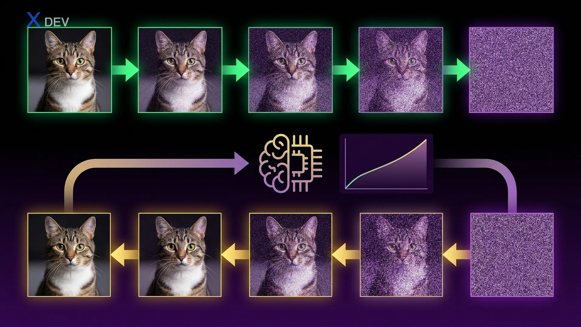
DDPM Overview — Two Processes
═════════════════════════════

  FORWARD DIFFUSION q(x_t | x_{t-1})         REVERSE DIFFUSION p_θ(x_{t-1} | x_t)
  ──────────────────────────────────         ───────────────────────────────────────

  x_0 ──► x_1 ──► x_2 ──►...──► x_T        x_T ──► x_{T-1} ──►...──► x_1 ──► x_0
  (clean)   +ε      +ε            (noise)   (noise)   U-Net     U-Net    (clean)

  ┌──────┐   ┌──────┐   ┌──────┐   ┌──────┐
  │ ████ │→  │ ▓▓▓▓ │→  │ ░░░░ │→  │ ···· │   Forward: add noise (fixed, no learning)
  │ ████ │   │ ▓▓▓▓ │   │ ░░░░ │   │ ···· │
  └──────┘   └──────┘   └──────┘   └──────┘
   t = 0      t = 100    t = 500    t = 1000

  ┌──────┐   ┌──────┐   ┌──────┐   ┌──────┐
  │ ···· │→  │ ░░░░ │→  │ ▓▓▓▓ │→  │ ████ │   Reverse: remove noise (learned by U-Net)
  │ ···· │   │ ░░░░ │   │ ▓▓▓▓ │   │ ████ │
  └──────┘   └──────┘   └──────┘   └──────┘
   t = 1000   t = 500    t = 100    t = 0
2. Forward Diffusion Process
2.1 Markov Chain Formulation
Forward diffusion is the process of gradually adding Gaussian noise to the original image x_0 over T timesteps. This is a Markov chain — each step depends only on the immediately preceding step:
q(x_{1:T} | x_0) = ∏_{t=1}^{T} q(x_t | x_{t-1})
At each timestep t, we add noise according to a Gaussian distribution:
q(x_t | x_{t-1}) = N(x_t;  √(1 - β_t) · x_{t-1},  β_t · I)
                         ▲ mean                    ▲ variance
Where β_t (beta) is the variance schedule — a small value that gradually increases from β_1 ≈ 0.0001 to β_T ≈ 0.02. It controls the amount of noise added at each step.
| Symbol | Meaning | Typical Value |
|---|---|---|
| β_t | Variance at timestep t | 0.0001 → 0.02 |
| α_t = 1 - β_t | Signal retention ratio | 0.9999 → 0.98 |
| ᾱ_t = ∏_{s=1}^{t} α_s | Cumulative signal retention | ≈1.0 → ≈0.0 |
| T | Total number of timesteps | 1000 (original DDPM) |
| ε | Standard Gaussian noise | ε ~ N(0, I) |
2.2 Closed-form: Jump Directly to Any Timestep
The key insight: we don't need to run sequentially through T forward steps. Thanks to the additive property of Gaussians, we have a closed-form solution to compute x_t directly from x_0:
q(x_t | x_0) = N(x_t;  √(ᾱ_t) · x_0,  (1 - ᾱ_t) · I)

Where:
  ᾱ_t = α_1 · α_2 · ... · α_t = ∏_{s=1}^{t} (1 - β_s)
This is extremely important for training — we can sample any timestep t without simulating the entire chain.
2.3 Reparameterization Trick
To sample x_t from the above distribution and backpropagate gradients, we use the reparameterization trick:
x_t = √(ᾱ_t) · x_0  +  √(1 - ᾱ_t) · ε      where ε ~ N(0, I)
      ────────────────   ──────────────────
      signal component    noise component
This formula says: at timestep t, the image x_t is a linear mixture of the original image (scaled by √ᾱ_t) and pure noise (scaled by √(1−ᾱ_t)). When t is small → ᾱ_t ≈ 1 → nearly all signal. When t is large → ᾱ_t ≈ 0 → nearly all noise.
Signal vs Noise across timesteps (T=1000, linear schedule)
══════════════════════════════════════════════════════════

  Signal: √(ᾱ_t)       Noise: √(1-ᾱ_t)
  1.0 ┤████████░░░░░░        0.0 ┤░░░░░░░░████████
      │████████░░░░░░            │░░░░░░░░████████
      │██████░░░░░░░░            │░░░░░░██████████
      │████░░░░░░░░░░            │░░░░████████████
      │██░░░░░░░░░░░░            │░░██████████████
  0.0 ┤░░░░░░░░░░░░░░        1.0 ┤████████████████
      └──────────────            └────────────────
       t=0        t=T             t=0          t=T

  At t ≈ T/2:  signal ≈ noise  (image is half clean, half noise)
  At t = T:    signal ≈ 0      (pure Gaussian noise)
2.4 Implementation: forward_diffusion()
import torch
import torch.nn as nn
import math

def forward_diffusion(x_0, t, sqrt_alpha_bar, sqrt_one_minus_alpha_bar):
    """
    Apply forward diffusion: x_t = sqrt(alpha_bar_t) * x_0 + sqrt(1 - alpha_bar_t) * eps

    Args:
        x_0: (B, C, H, W) — clean images
        t: (B,) — timestep indices (0-indexed)
        sqrt_alpha_bar: (T,) — precomputed sqrt(ᾱ_t)
        sqrt_one_minus_alpha_bar: (T,) — precomputed sqrt(1 - ᾱ_t)
    Returns:
        x_t: (B, C, H, W) — noisy images at timestep t
        noise: (B, C, H, W) — the noise that was added (needed for loss)
    """
    # Sample Gaussian noise
    noise = torch.randn_like(x_0)

    # Gather coefficients for each sample in batch
    # (B,) -> (B, 1, 1, 1) for broadcasting with (B, C, H, W)
    s_alpha = sqrt_alpha_bar[t].view(-1, 1, 1, 1)
    s_one_minus = sqrt_one_minus_alpha_bar[t].view(-1, 1, 1, 1)

    # Reparameterization: x_t = sqrt(ᾱ_t) * x_0 + sqrt(1-ᾱ_t) * ε
    x_t = s_alpha * x_0 + s_one_minus * noise

    return x_t, noise
Exam tip: Note the
.view(-1, 1, 1, 1)— this is a mandatory pattern when gathering scalar coefficients then broadcasting with a 4D tensor. Forgetting to reshape will cause shape mismatches. The assessment frequently tests exactly this point.
3. Noise Scheduling
3.1 Linear Schedule (Original DDPM)
The original DDPM paper uses a linear schedule: β increases linearly from β_1 = 0.0001 to β_T = 0.02 over T = 1000 steps.
def linear_beta_schedule(T, beta_start=1e-4, beta_end=0.02):
    """
    Linear variance schedule: β_t increases linearly from beta_start to beta_end.
    Original DDPM (Ho et al. 2020).
    """
    return torch.linspace(beta_start, beta_end, T)


def precompute_schedule(betas):
    """Precompute all coefficients from beta schedule."""
    alphas = 1.0 - betas                          # α_t = 1 - β_t
    alpha_bar = torch.cumprod(alphas, dim=0)       # ᾱ_t = ∏ α_s
    sqrt_alpha_bar = torch.sqrt(alpha_bar)         # √(ᾱ_t)
    sqrt_one_minus_alpha_bar = torch.sqrt(1.0 - alpha_bar)  # √(1 - ᾱ_t)
    sqrt_alpha = torch.sqrt(alphas)                # √(α_t)  — for reverse step

    return {
        'betas': betas,
        'alphas': alphas,
        'alpha_bar': alpha_bar,
        'sqrt_alpha_bar': sqrt_alpha_bar,
        'sqrt_one_minus_alpha_bar': sqrt_one_minus_alpha_bar,
        'sqrt_alpha': sqrt_alpha,
    }

# Usage
T = 1000
schedule = precompute_schedule(linear_beta_schedule(T))
3.2 Cosine Schedule (Improved DDPM)
Problem with linear schedule: ᾱ_t drops too quickly in the middle → the image gets destroyed too early, causing information loss. Cosine schedule (Nichol & Dhariwal 2021) fixes this by designing ᾱ_t using a cosine function — smoother decay, especially better for high-resolution images.
def cosine_beta_schedule(T, s=0.008):
    """
    Cosine variance schedule (Nichol & Dhariwal 2021).
    Designs alpha_bar directly via cosine function, then derives betas.
    The 's' offset prevents beta from being too small near t=0.
    """
    steps = torch.arange(T + 1, dtype=torch.float32)
    # f(t) = cos( (t/T + s) / (1+s) * π/2 )²
    f_t = torch.cos(((steps / T) + s) / (1 + s) * (math.pi / 2)) ** 2
    alpha_bar = f_t / f_t[0]  # normalize so alpha_bar[0] = 1

    # Derive betas from alpha_bar: β_t = 1 - ᾱ_t / ᾱ_{t-1}
    betas = 1 - (alpha_bar[1:] / alpha_bar[:-1])
    betas = torch.clamp(betas, min=1e-5, max=0.999)  # numerical stability

    return betas
| Feature | Linear Schedule | Cosine Schedule |
|---|---|---|
| ᾱ_t at t=T/2 | ≈ 0.05 (near 0) | ≈ 0.50 (still has signal) |
| Signal destruction | Fast, aggressive | Smooth, gradual |
| High-resolution images | Poor (loses detail early) | Much better |
| Original paper | DDPM (Ho 2020) | Improved DDPM (Nichol 2021) |
| Used in Stable Diffusion | No | Yes (variant) |
| NVIDIA DLI focus | Implement in lab | Understand concept, compare |
ᾱ_t Comparison: Linear vs Cosine (T=1000)
══════════════════════════════════════════

  ᾱ_t
  1.0 ┤C C C C L
      │C C C   L
  0.8 ┤  C C    L
      │    C     L
  0.6 ┤    C      L
      │     C      L
  0.4 ┤      C      L
      │       C      L
  0.2 ┤        C      L
      │         C C    L L
  0.0 ┤            C C C L L L L
      └─────────────────────────
       t=0    t=250   t=500  t=750  t=1000

  L = Linear schedule (drops fast mid-range)
  C = Cosine schedule (smooth decay, retains signal longer)

  Key: Cosine retains signal longer → better generation quality
Exam tip: Questions will ask "why is cosine schedule better than linear?" — Answer: because cosine retains signal longer at mid-range timesteps, avoiding premature information destruction. With linear, ᾱ_{T/2} ≈ 0.05 means 95% of signal is already lost halfway through the process.
4. Reverse Diffusion Process
4.1 Goal: Learn the Reverse Distribution
Reverse diffusion is the opposite process — starting from pure noise x_T ~ N(0, I) and gradually denoising back to a clean image x_0. This is the learned part — U-Net will learn:
p_θ(x_{t-1} | x_t)  =  N(x_{t-1};  μ_θ(x_t, t),  σ²_t · I)
                              ▲ predicted mean      ▲ fixed variance
Instead of predicting the mean μ directly, DDPM takes a more elegant approach: the model predicts the noise ε that was added to the image. From the predicted ε̂, we derive the mean:
μ_θ(x_t, t) = ────────── · ( x_t  −  ──────────── · ε_θ(x_t, t) )
                  1                      1 - α_t
               ───────                ──────────────
                √(α_t)                 √(1 - ᾱ_t)

Compact form:
                    1              (1 - α_t)
μ_θ(x_t, t) = ───────── · (x_t − ─────────── · ε_θ(x_t, t))
                √(α_t)           √(1 - ᾱ_t)
4.2 Sampling Algorithm
The sampling algorithm goes from x_T back to x_0:
Algorithm: DDPM Sampling
════════════════════════
Input: trained model ε_θ, noise schedule {β_t, α_t, ᾱ_t}

1. Sample x_T ~ N(0, I)                  ← start from pure noise
2. For t = T, T-1, ..., 1:
   a. If t > 1: sample z ~ N(0, I)
      Else:     z = 0                     ← no noise at final step
   b. ε̂ = ε_θ(x_t, t)                    ← U-Net predicts noise
   c. μ = (1/√α_t) · (x_t − ((1-α_t)/√(1-ᾱ_t)) · ε̂)
   d. x_{t-1} = μ + σ_t · z              ← denoise one step
      where σ_t = √(β_t)                 ← simplified variance

3. Return x_0
Reverse Process Visualization
═════════════════════════════

  x_T (pure noise)              x_0 (clean image)
  ┌──────────┐                  ┌──────────┐
  │ ·:·:·:·: │   U-Net × T     │ ████████ │
  │ :·:·:·:· │  ──────────►    │ ██    ██ │
  │ ·:·:·:·: │   denoise       │ ██    ██ │
  │ :·:·:·:· │   iteratively   │ ████████ │
  └──────────┘                  └──────────┘

  Step-by-step (T=1000):
  t=1000      t=750       t=500       t=250       t=0
  ┌──────┐   ┌──────┐   ┌──────┐   ┌──────┐   ┌──────┐
  │ ···· │ → │ ░··░ │ → │ ░▓▓░ │ → │ ▓██▓ │ → │ ████ │
  │ ···· │   │ ·░░· │   │ ▓░░▓ │   │ █▓▓█ │   │ █  █ │
  │ ···· │   │ ·░░· │   │ ▓░░▓ │   │ █▓▓█ │   │ █  █ │
  │ ···· │   │ ░··░ │   │ ░▓▓░ │   │ ▓██▓ │   │ ████ │
  └──────┘   └──────┘   └──────┘   └──────┘   └──────┘
  noise only   structure   shape      details    clean!
               emerges     forms      sharpen
4.3 Implementation: Reverse Sampling Loop
@torch.no_grad()
def sample_ddpm(model, shape, schedule, device='cuda'):
    """
    DDPM sampling: generate images from pure noise.

    Args:
        model: trained U-Net noise predictor ε_θ
        shape: (B, C, H, W) — output shape
        schedule: dict with 'betas', 'alphas', 'alpha_bar', etc.
        device: torch device
    Returns:
        x_0: (B, C, H, W) — generated images
    """
    T = len(schedule['betas'])
    betas = schedule['betas'].to(device)
    alphas = schedule['alphas'].to(device)
    alpha_bar = schedule['alpha_bar'].to(device)
    sqrt_alpha = schedule['sqrt_alpha'].to(device)
    sqrt_one_minus_alpha_bar = schedule['sqrt_one_minus_alpha_bar'].to(device)

    # Step 1: Start from pure Gaussian noise
    x_t = torch.randn(shape, device=device)

    # Step 2: Iteratively denoise from t=T-1 down to t=0
    for t in reversed(range(T)):
        t_batch = torch.full((shape[0],), t, device=device, dtype=torch.long)

        # (a) Predict noise using U-Net
        eps_pred = model(x_t, t_batch)

        # (b) Compute predicted mean μ_θ
        #     μ = (1/√α_t) * (x_t - (1-α_t)/√(1-ᾱ_t) * ε̂)
        coeff_xt = 1.0 / sqrt_alpha[t]
        coeff_eps = (1.0 - alphas[t]) / sqrt_one_minus_alpha_bar[t]
        mu = coeff_xt * (x_t - coeff_eps * eps_pred)

        # (c) Add noise (except at t=0)
        if t > 0:
            sigma = torch.sqrt(betas[t])
            z = torch.randn_like(x_t)
            x_t = mu + sigma * z
        else:
            x_t = mu  # final step: no noise added

    return x_t
Exam tip: The two most common mistakes in the sampling loop: (1) forgetting
@torch.no_grad()→ uses 3-4x more VRAM, OOM crash. (2) Adding noise at step t=0 → output image remains noisy. Always checkif t > 0before adding z.
5. Training Objective: Simplified ELBO Loss
5.1 From ELBO to Simplified Loss
Theoretically, DDPM optimizes the variational lower bound (ELBO) of the log-likelihood. However, Ho et al. discovered that a simplified loss works better in practice:
Full ELBO Loss (theoretical):
L_vlb = L_0 + L_1 + ... + L_{T-1} + L_T
      = ∑_t KL(q(x_{t-1}|x_t,x_0) || p_θ(x_{t-1}|x_t))

Simplified Loss (practical — DDPM paper):
L_simple = E_{t ~ U{1,T}, x_0, ε} [ || ε − ε_θ(x_t, t) ||² ]

Meaning:
  - Sample a random timestep t
  - Create x_t from x_0 via forward diffusion
  - U-Net predicts noise ε̂ = ε_θ(x_t, t)
  - Loss = MSE between actual noise (ε) and predicted noise (ε̂)
This is exactly why you need to return noise from forward_diffusion() — it serves as the ground truth label for training.
5.2 Training Algorithm
Algorithm: DDPM Training
════════════════════════
Repeat until convergence:
  1. Sample x_0 ~ q(x_0)              ← batch from dataset
  2. Sample t ~ Uniform({1, ..., T})   ← random timestep per sample
  3. Sample ε ~ N(0, I)               ← target noise
  4. Compute x_t = √(ᾱ_t)·x_0 + √(1−ᾱ_t)·ε    ← forward diffusion
  5. Compute ε̂ = ε_θ(x_t, t)          ← U-Net predicts noise
  6. Loss = MSE(ε, ε̂)                 ← compare real vs predicted noise
  7. Backprop & update θ
5.3 Implementation: Complete Training Loop
def train_ddpm(model, dataloader, schedule, epochs=100, lr=2e-4, device='cuda'):
    """
    Full DDPM training loop.

    Args:
        model: U-Net noise predictor
        dataloader: yields (images, labels) batches
        schedule: precomputed noise schedule dict
        epochs: number of training epochs
        lr: learning rate
        device: torch device
    """
    optimizer = torch.optim.Adam(model.parameters(), lr=lr)
    loss_fn = nn.MSELoss()
    T = len(schedule['betas'])

    sqrt_alpha_bar = schedule['sqrt_alpha_bar'].to(device)
    sqrt_one_minus_alpha_bar = schedule['sqrt_one_minus_alpha_bar'].to(device)

    model.train()
    for epoch in range(epochs):
        epoch_loss = 0.0
        for batch_idx, (x_0, _) in enumerate(dataloader):
            x_0 = x_0.to(device)
            B = x_0.shape[0]

            # Step 2: Sample random timesteps
            t = torch.randint(0, T, (B,), device=device)

            # Steps 3-4: Forward diffusion (sample noise + compute x_t)
            x_t, noise = forward_diffusion(
                x_0, t, sqrt_alpha_bar, sqrt_one_minus_alpha_bar
            )

            # Step 5: Predict noise
            noise_pred = model(x_t, t)

            # Step 6: Compute loss
            loss = loss_fn(noise_pred, noise)

            # Step 7: Backprop
            optimizer.zero_grad()
            loss.backward()
            optimizer.step()

            epoch_loss += loss.item()

        avg_loss = epoch_loss / len(dataloader)
        if (epoch + 1) % 10 == 0:
            print(f"Epoch {epoch+1}/{epochs}, Loss: {avg_loss:.4f}")
| Training Component | Role | Corresponding Code |
|---|---|---|
| x_0 from dataset | Clean image input | x_0 = batch[0].to(device) |
| t ~ Uniform | Random timestep | torch.randint(0, T, (B,)) |
| ε ~ N(0,I) | Target noise | torch.randn_like(x_0) |
| x_t via reparameterization | Noisy image | forward_diffusion(...) |
| ε_θ(x_t, t) | U-Net prediction | model(x_t, t) |
| MSE(ε, ε̂) | Simplified loss | nn.MSELoss()(pred, target) |
Exam tip: In the assessment, you will have to write the training loop from scratch. The order of steps is critical: forward diffusion → predict → loss → backprop. If you place
optimizer.zero_grad()in the wrong position or forgetloss.backward(), the model won't learn — and you'll lose points.
6. Classifier-Free Diffusion Guidance (CFG)
6.1 Conditional Generation and CFG
Vanilla DDPM generates images unconditionally. To generate images according to a condition (class label, text prompt), we need conditional generation. Classifier-Free Guidance (CFG) is the most elegant approach:
Classifier-Free Guidance
═════════════════════════

  Training: Model receives condition c, but randomly drops c → ∅ with probability p_uncond
  ┌──────────────────────────────────────┐
  │  if random() < p_uncond (e.g. 0.1): │
  │      c = ∅  (null / empty)           │    ← 10% unconditional
  │  ε̂ = ε_θ(x_t, t, c)                 │
  └──────────────────────────────────────┘

  Inference: Combine conditional & unconditional predictions
  ┌──────────────────────────────────────────────────────────────┐
  │  ε̂_uncond = ε_θ(x_t, t, ∅)           ← unconditional pred  │
  │  ε̂_cond   = ε_θ(x_t, t, c)           ← conditional pred    │
  │                                                              │
  │  ε̂_guided = ε̂_uncond + w · (ε̂_cond − ε̂_uncond)             │
  │              ▲                 ▲ guidance direction           │
  │              baseline          amplified by scale w           │
  └──────────────────────────────────────────────────────────────┘

  w = guidance scale:
    w = 1.0  → standard conditional (no guidance)
    w = 7.5  → typical value (Stable Diffusion default)
    w = 20   → very strong guidance → faithful but less diverse
    w = 0.0  → purely unconditional
6.2 Guidance Scale Trade-off
| Guidance Scale w | Quality | Diversity | Condition Fidelity | Use Case |
|---|---|---|---|---|
| 0.0 | Low | Very high | None (unconditional) | Exploration |
| 1.0 | Medium | High | Standard | No guidance |
| 3.0 – 5.0 | Good | Medium | Good | Balanced generation |
| 7.0 – 8.5 | Very good | Lower | Very good | Default Stable Diffusion |
| 15.0 – 20.0 | Oversaturated | Very low | Excessive | Artistic, stylized |
6.3 Implementation: CFG Training & Sampling
def train_ddpm_cfg(model, dataloader, schedule, epochs=100,
                   lr=2e-4, p_uncond=0.1, num_classes=10, device='cuda'):
    """
    DDPM training with Classifier-Free Guidance.
    Model takes (x_t, t, class_label) as input.
    During training, randomly replace class_label with null_class.
    """
    optimizer = torch.optim.Adam(model.parameters(), lr=lr)
    loss_fn = nn.MSELoss()
    T = len(schedule['betas'])
    null_class = num_classes  # use num_classes as "no class" token

    sqrt_ab = schedule['sqrt_alpha_bar'].to(device)
    sqrt_omab = schedule['sqrt_one_minus_alpha_bar'].to(device)

    model.train()
    for epoch in range(epochs):
        for x_0, labels in dataloader:
            x_0, labels = x_0.to(device), labels.to(device)
            B = x_0.shape[0]

            # Random timestep
            t = torch.randint(0, T, (B,), device=device)

            # CFG: randomly drop condition
            mask = torch.rand(B, device=device) < p_uncond
            labels_cfg = labels.clone()
            labels_cfg[mask] = null_class  # replace with null token

            # Forward diffusion
            x_t, noise = forward_diffusion(x_0, t, sqrt_ab, sqrt_omab)

            # Predict noise (conditioned on possibly-null label)
            noise_pred = model(x_t, t, labels_cfg)

            # Loss
            loss = loss_fn(noise_pred, noise)
            optimizer.zero_grad()
            loss.backward()
            optimizer.step()


@torch.no_grad()
def sample_ddpm_cfg(model, shape, schedule, class_label, guidance_scale=7.5,
                    num_classes=10, device='cuda'):
    """
    DDPM sampling with Classifier-Free Guidance.

    ε̂_guided = ε̂_uncond + w * (ε̂_cond - ε̂_uncond)

    Args:
        class_label: (B,) — target class for each sample
        guidance_scale: w — higher = more faithful to condition
    """
    T = len(schedule['betas'])
    betas = schedule['betas'].to(device)
    alphas = schedule['alphas'].to(device)
    alpha_bar = schedule['alpha_bar'].to(device)
    sqrt_alpha = schedule['sqrt_alpha'].to(device)
    sqrt_omab = schedule['sqrt_one_minus_alpha_bar'].to(device)
    null_class = num_classes

    x_t = torch.randn(shape, device=device)
    class_label = class_label.to(device)
    null_label = torch.full_like(class_label, null_class)

    for t in reversed(range(T)):
        t_batch = torch.full((shape[0],), t, device=device, dtype=torch.long)

        # Two forward passes: conditional + unconditional
        eps_cond = model(x_t, t_batch, class_label)    # ε_θ(x_t, t, c)
        eps_uncond = model(x_t, t_batch, null_label)   # ε_θ(x_t, t, ∅)

        # CFG formula
        eps_guided = eps_uncond + guidance_scale * (eps_cond - eps_uncond)

        # Compute mean
        coeff_xt = 1.0 / sqrt_alpha[t]
        coeff_eps = (1.0 - alphas[t]) / sqrt_omab[t]
        mu = coeff_xt * (x_t - coeff_eps * eps_guided)

        # Denoise step
        if t > 0:
            sigma = torch.sqrt(betas[t])
            x_t = mu + sigma * torch.randn_like(x_t)
        else:
            x_t = mu

    return x_t
Exam tip: CFG requires two forward passes per sampling step — one conditional, one unconditional. This is why sampling with CFG is twice as slow. In the DLI lab, if you only run one forward pass, guidance will have no effect — output will be the same as unconditional.
7. Cheat Sheet: DDPM Formulas Summary
| Formula | Meaning | Where Used |
|---|---|---|
| x_t = √ᾱ_t · x_0 + √(1−ᾱ_t) · ε | Forward diffusion (closed-form) | Training: create x_t from x_0 |
| ε̂ = ε_θ(x_t, t) | U-Net predicts noise | Training: output | Sampling: denoise |
| L = MSE(ε, ε̂) | Simplified ELBO loss | Training: compute loss |
| μ = (1/√α_t)(x_t − (1−α_t)/√(1−ᾱ_t) · ε̂) | Predicted mean for reverse step | Sampling: compute μ_θ |
| x_{t−1} = μ + √β_t · z | Sampling step (z=0 when t=0) | Sampling: denoise one step |
| ε̂ = ε̂_∅ + w(ε̂_c − ε̂_∅) | CFG guidance formula | Conditional sampling |
DDPM Pipeline Summary
═════════════════════

  ┌─────────────────────────────────────────────────────────┐
  │                      TRAINING                           │
  │                                                         │
  │  x_0 ──[forward_diffusion]──► x_t ──[U-Net]──► ε̂      │
  │   │         ↑                                    │      │
  │   └─── t,ε (random) ───────────────── MSE(ε, ε̂) │      │
  │                                         │               │
  │                                    backprop             │
  └─────────────────────────────────────────────────────────┘

  ┌─────────────────────────────────────────────────────────┐
  │                     SAMPLING                            │
  │                                                         │
  │  x_T ──► [U-Net] ──► ε̂ ──► μ_θ ──► x_{T-1}           │
  │                                       │                 │
  │         [U-Net] ──► ε̂ ──► μ_θ ──► x_{T-2}             │
  │                                       │                 │
  │         ...repeat T times...          │                 │
  │                                       ▼                 │
  │                                      x_0 (generated!)  │
  └─────────────────────────────────────────────────────────┘

  ┌─────────────────────────────────────────────────────────┐
  │                   CFG SAMPLING                          │
  │                                                         │
  │  At each step t:                                        │
  │    ε̂_∅ = UNet(x_t, t, null)      ← unconditional      │
  │    ε̂_c = UNet(x_t, t, class)     ← conditional        │
  │    ε̂ = ε̂_∅ + w · (ε̂_c − ε̂_∅)   ← guided prediction  │
  │    x_{t-1} = denoise(x_t, ε̂)                          │
  └─────────────────────────────────────────────────────────┘
8. Practice Questions
5 coding questions — try implementing before checking the answers.
Q1: Implement forward_diffusion(x_0, t, noise_schedule) → x_t, noise
Write the forward_diffusion function that takes a batch of images x_0, a tensor of timesteps t, and a dictionary noise_schedule containing precomputed coefficients. Return x_t and the noise ε that was used.
def forward_diffusion(x_0, t, noise_schedule):
    """
    Args:
        x_0: (B, C, H, W) — clean images, normalized to [-1, 1]
        t: (B,) — integer timestep indices
        noise_schedule: dict with keys:
            'sqrt_alpha_bar': (T,) tensor
            'sqrt_one_minus_alpha_bar': (T,) tensor
    Returns:
        x_t: (B, C, H, W) — noisy images
        noise: (B, C, H, W) — the Gaussian noise added
    """
    # TODO: Implement forward diffusion using reparameterization trick
    pass
Show Answer Q1
def forward_diffusion(x_0, t, noise_schedule):
    sqrt_alpha_bar = noise_schedule['sqrt_alpha_bar']
    sqrt_one_minus_alpha_bar = noise_schedule['sqrt_one_minus_alpha_bar']

    # Sample noise ε ~ N(0, I)
    noise = torch.randn_like(x_0)

    # Gather coefficients for batch and reshape for broadcasting
    # (B,) → (B, 1, 1, 1)
    s_ab = sqrt_alpha_bar[t].view(-1, 1, 1, 1)
    s_omab = sqrt_one_minus_alpha_bar[t].view(-1, 1, 1, 1)

    # Reparameterization trick:
    # x_t = √(ᾱ_t) * x_0 + √(1 - ᾱ_t) * ε
    x_t = s_ab * x_0 + s_omab * noise

    return x_t, noise
Explanation: Three key steps: (1) sample noise with the same shape as x_0 using torch.randn_like, (2) gather coefficients by index t then reshape with .view(-1, 1, 1, 1) for 4D broadcasting, (3) apply the reparameterization trick. Note that we must return the noise as well because the training loop needs it as the target for MSE loss.
Q2: Implement reverse diffusion sampling loop
Write the sample_ddpm function that generates new images from pure noise by iterating through reverse diffusion steps. The model has already been trained.
@torch.no_grad()
def sample_ddpm(model, n_samples, img_channels, img_size, schedule, device):
    """
    Args:
        model: trained U-Net, expects (x_t, t_batch) → predicted noise
        n_samples: int — number of images to generate
        img_channels: int — e.g., 1 for MNIST
        img_size: int — e.g., 28
        schedule: dict with 'betas', 'alphas', 'alpha_bar',
                  'sqrt_alpha', 'sqrt_one_minus_alpha_bar'
    Returns:
        images: (n_samples, C, H, W) — generated images
    """
    # TODO: Implement the full DDPM sampling algorithm
    pass
Show Answer Q2
@torch.no_grad()
def sample_ddpm(model, n_samples, img_channels, img_size, schedule, device):
    T = len(schedule['betas'])
    betas = schedule['betas'].to(device)
    alphas = schedule['alphas'].to(device)
    sqrt_alpha = schedule['sqrt_alpha'].to(device)
    sqrt_omab = schedule['sqrt_one_minus_alpha_bar'].to(device)

    shape = (n_samples, img_channels, img_size, img_size)

    # Start from pure noise x_T ~ N(0, I)
    x_t = torch.randn(shape, device=device)

    for t in reversed(range(T)):
        t_batch = torch.full((n_samples,), t, device=device, dtype=torch.long)

        # U-Net predicts noise
        eps_pred = model(x_t, t_batch)

        # Compute predicted mean:
        # μ_θ = (1/√α_t) * (x_t − ((1−α_t) / √(1−ᾱ_t)) * ε̂)
        coeff_xt = 1.0 / sqrt_alpha[t]
        coeff_eps = (1.0 - alphas[t]) / sqrt_omab[t]
        mu = coeff_xt * (x_t - coeff_eps * eps_pred)

        # Sample x_{t-1}: add noise for t > 0, otherwise return mean
        if t > 0:
            sigma = torch.sqrt(betas[t])
            z = torch.randn_like(x_t)
            x_t = mu + sigma * z
        else:
            x_t = mu

    return x_t
Explanation: The sampling loop runs in reverse from t=T-1 down to t=0. At each step: (1) U-Net predicts noise ε̂, (2) compute mean μ_θ using the DDPM formula, (3) add noise z if t > 0 (stochastic sampling). Critical: use @torch.no_grad() to avoid accumulating gradients over 1000 steps — this would cause OOM. Step t=0 does not add noise because it is the final output.
Q3: Debug — model outputs black images
A student implemented reverse sampling but the result is always a black image (near 0). Find the bug in the code below:
@torch.no_grad()
def buggy_sample(model, shape, schedule, device):
    T = len(schedule['betas'])
    betas = schedule['betas'].to(device)
    alphas = schedule['alphas'].to(device)
    sqrt_alpha = schedule['sqrt_alpha'].to(device)
    sqrt_omab = schedule['sqrt_one_minus_alpha_bar'].to(device)

    x_t = torch.randn(shape, device=device)

    for t in reversed(range(T)):
        t_batch = torch.full((shape[0],), t, device=device, dtype=torch.long)
        eps_pred = model(x_t, t_batch)

        # BUG IS HERE — find it!
        coeff_xt = 1.0 / sqrt_alpha[t]
        coeff_eps = (1.0 - alphas[t]) / sqrt_omab[t]
        mu = coeff_xt * (x_t + coeff_eps * eps_pred)  # line A

        if t > 0:
            sigma = torch.sqrt(betas[t])
            x_t = mu + sigma * torch.randn_like(x_t)
        else:
            x_t = mu

    return x_t
Show Answer Q3
Bug: The line computing μ uses + instead of − before coeff_eps * eps_pred.
# BUG (line A):
mu = coeff_xt * (x_t + coeff_eps * eps_pred)   # ← WRONG: + instead of -

# FIX:
mu = coeff_xt * (x_t - coeff_eps * eps_pred)   # ← CORRECT: subtract noise
Explanation: The DDPM reverse mean formula is μ = (1/√α_t)(x_t − ((1−α_t)/√(1−ᾱ_t)) · ε̂). The minus sign is the essence of "denoising" — we subtract the predicted noise. When using a plus sign, we actually add more noise instead of removing it → over 1000 steps, the image gets neutralized (oscillates around 0) → output is near 0 (black). This is a subtle bug because the code still runs without errors, the output still has the correct shape — only the values are wrong.
Q4: Implement CFG sampling with guidance scale
The model has been trained with condition dropout. Write a sampling function with Classifier-Free Guidance.
@torch.no_grad()
def sample_cfg(model, shape, schedule, class_labels, guidance_scale,
               num_classes, device):
    """
    Args:
        model: U-Net with signature model(x_t, t, class_label) → noise
        shape: (B, C, H, W)
        class_labels: (B,) — target class indices
        guidance_scale: float w — e.g. 7.5
        num_classes: int — total classes (null_class = num_classes)
    Returns:
        images: (B, C, H, W)
    """
    # TODO: Implement CFG sampling
    # Hint: two forward passes per step — conditional & unconditional
    pass
Show Answer Q4
@torch.no_grad()
def sample_cfg(model, shape, schedule, class_labels, guidance_scale,
               num_classes, device):
    T = len(schedule['betas'])
    betas = schedule['betas'].to(device)
    alphas = schedule['alphas'].to(device)
    sqrt_alpha = schedule['sqrt_alpha'].to(device)
    sqrt_omab = schedule['sqrt_one_minus_alpha_bar'].to(device)
    null_class = num_classes

    x_t = torch.randn(shape, device=device)
    class_labels = class_labels.to(device)
    null_labels = torch.full_like(class_labels, null_class)

    for t in reversed(range(T)):
        t_batch = torch.full((shape[0],), t, device=device, dtype=torch.long)

        # Two forward passes
        eps_uncond = model(x_t, t_batch, null_labels)   # ε_θ(x_t, t, ∅)
        eps_cond = model(x_t, t_batch, class_labels)    # ε_θ(x_t, t, c)

        # CFG: ε̂ = ε_uncond + w * (ε_cond - ε_uncond)
        eps_guided = eps_uncond + guidance_scale * (eps_cond - eps_uncond)

        # Reverse step with guided noise prediction
        coeff_xt = 1.0 / sqrt_alpha[t]
        coeff_eps = (1.0 - alphas[t]) / sqrt_omab[t]
        mu = coeff_xt * (x_t - coeff_eps * eps_guided)

        if t > 0:
            sigma = torch.sqrt(betas[t])
            x_t = mu + sigma * torch.randn_like(x_t)
        else:
            x_t = mu

    return x_t
Explanation: CFG sampling differs from standard sampling in that at each step we run two U-Net forward passes: (1) unconditional with null_class, (2) conditional with the actual class. Then combine: ε̂ = ε̂_∅ + w·(ε̂_c − ε̂_∅). When w=1.0 → standard conditional (no guidance). When w>1.0 → amplifies the difference between conditional and unconditional → sharper images but less diverse. null_class is typically = num_classes (an index outside the real classes).
Q5: Compare linear vs cosine schedule — when does ᾱ_t drop below 0.01?
Write code to compute and compare: with T=1000, at which timestep does ᾱ_t drop below 0.01 for each schedule? What does this mean for generation quality?
def compare_schedules(T=1000):
    """
    Compute alpha_bar for both linear and cosine schedules.
    Find the timestep where alpha_bar drops below 0.01 for each.
    Print comparison results.
    """
    # TODO: implement using linear_beta_schedule() and cosine_beta_schedule()
    pass
Show Answer Q5
import torch
import math

def linear_beta_schedule(T, beta_start=1e-4, beta_end=0.02):
    return torch.linspace(beta_start, beta_end, T)

def cosine_beta_schedule(T, s=0.008):
    steps = torch.arange(T + 1, dtype=torch.float32)
    f_t = torch.cos(((steps / T) + s) / (1 + s) * (math.pi / 2)) ** 2
    alpha_bar = f_t / f_t[0]
    betas = 1 - (alpha_bar[1:] / alpha_bar[:-1])
    return torch.clamp(betas, min=1e-5, max=0.999)

def compare_schedules(T=1000):
    # Linear schedule
    betas_lin = linear_beta_schedule(T)
    alphas_lin = 1.0 - betas_lin
    alpha_bar_lin = torch.cumprod(alphas_lin, dim=0)

    # Cosine schedule
    betas_cos = cosine_beta_schedule(T)
    alphas_cos = 1.0 - betas_cos
    alpha_bar_cos = torch.cumprod(alphas_cos, dim=0)

    # Find where alpha_bar < 0.01
    threshold = 0.01
    t_lin = (alpha_bar_lin < threshold).nonzero(as_tuple=True)[0][0].item()
    t_cos = (alpha_bar_cos < threshold).nonzero(as_tuple=True)[0][0].item()

    print(f"Linear schedule: ᾱ_t < {threshold} at t = {t_lin}")
    print(f"  ᾱ at t=250: {alpha_bar_lin[250]:.4f}")
    print(f"  ᾱ at t=500: {alpha_bar_lin[500]:.4f}")
    print(f"  ᾱ at t=750: {alpha_bar_lin[750]:.6f}")
    print()
    print(f"Cosine schedule: ᾱ_t < {threshold} at t = {t_cos}")
    print(f"  ᾱ at t=250: {alpha_bar_cos[250]:.4f}")
    print(f"  ᾱ at t=500: {alpha_bar_cos[500]:.4f}")
    print(f"  ᾱ at t=750: {alpha_bar_cos[750]:.4f}")
    print()
    print(f"Difference: cosine retains signal for {t_cos - t_lin} more timesteps")

compare_schedules()
# Output (approximate):
# Linear schedule: ᾱ_t < 0.01 at t ≈ 650
#   ᾱ at t=250: 0.6766
#   ᾱ at t=500: 0.0473
#   ᾱ at t=750: 0.000014
#
# Cosine schedule: ᾱ_t < 0.01 at t ≈ 940
#   ᾱ at t=250: 0.8536
#   ᾱ at t=500: 0.5000
#   ᾱ at t=750: 0.1464
#
# Difference: cosine retains signal for ~290 more timesteps
Explanation: The linear schedule destroys signal early — ᾱ_t < 0.01 around t≈650, meaning the final 35% of the chain is nearly useless (noise is practically pure). Cosine keeps ᾱ_t > 0.01 until t≈940, making more efficient use of all T steps. Pay special attention: at t=500 (midpoint of the chain), linear only has ᾱ≈0.05 (5% signal) while cosine still has ᾱ≈0.50 (50% signal). This explains why cosine produces better generation quality — the model gets useful gradients from more timesteps, without wasted computation in the pure noise region.
Exam tip: In the DLI assessment, questions about noise schedules typically require you to explain why one schedule is better. Key insight: a good schedule should distribute signal destruction evenly across all timesteps — not too fast (linear), not too slow. Cosine achieves this by designing ᾱ_t directly rather than β_t.