1. Giới thiệu: Toán học đằng sau Diffusion Models
Bài này là phần khó nhất trong toàn bộ khoá DLI. Bạn sẽ đi sâu vào nền tảng toán học của Denoising Diffusion Probabilistic Models (DDPM) — paper gốc từ Ho et al. (2020). Mọi diffusion model hiện đại (Stable Diffusion, DALL·E, Imagen) đều dựa trên framework này.
Bài trước bạn đã xây xong U-Net — kiến trúc backbone. Giờ bạn sẽ hiểu chính xác U-Net học cái gì, bằng cách nào, và tại sao nó hoạt động.
Exam tip: NVIDIA DLI assessment yêu cầu bạn implement cả forward diffusion, reverse sampling, và training loop từ đầu. Hiểu rõ từng công thức và cách chúng map sang code PyTorch là bắt buộc — không chỉ chạy code mẫu.
DDPM Overview — Two Processes
═════════════════════════════

  FORWARD DIFFUSION q(x_t | x_{t-1})         REVERSE DIFFUSION p_θ(x_{t-1} | x_t)
  ──────────────────────────────────         ───────────────────────────────────────

  x_0 ──► x_1 ──► x_2 ──►...──► x_T        x_T ──► x_{T-1} ──►...──► x_1 ──► x_0
  (clean)   +ε      +ε            (noise)   (noise)   U-Net     U-Net    (clean)

  ┌──────┐   ┌──────┐   ┌──────┐   ┌──────┐
  │ ████ │→  │ ▓▓▓▓ │→  │ ░░░░ │→  │ ···· │   Forward: add noise (fixed, no learning)
  │ ████ │   │ ▓▓▓▓ │   │ ░░░░ │   │ ···· │
  └──────┘   └──────┘   └──────┘   └──────┘
   t = 0      t = 100    t = 500    t = 1000

  ┌──────┐   ┌──────┐   ┌──────┐   ┌──────┐
  │ ···· │→  │ ░░░░ │→  │ ▓▓▓▓ │→  │ ████ │   Reverse: remove noise (learned by U-Net)
  │ ···· │   │ ░░░░ │   │ ▓▓▓▓ │   │ ████ │
  └──────┘   └──────┘   └──────┘   └──────┘
   t = 1000   t = 500    t = 100    t = 0
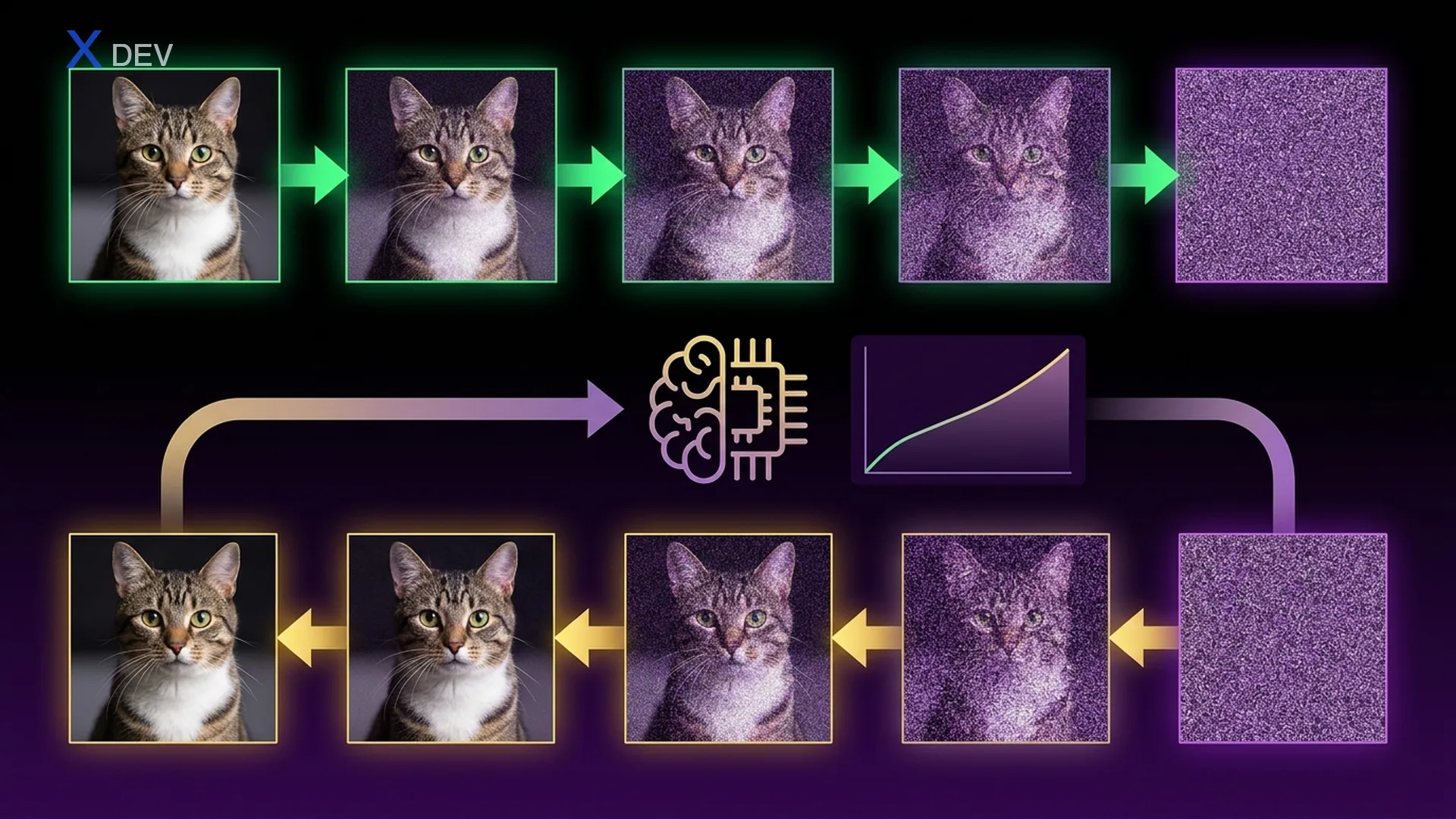
2. Forward Diffusion Process
2.1 Markov Chain formulation
Forward diffusion là quá trình dần dần thêm Gaussian noise vào ảnh gốc x_0 qua T timesteps. Đây là một Markov chain — mỗi bước chỉ phụ thuộc vào bước ngay trước đó:
q(x_{1:T} | x_0) = ∏_{t=1}^{T} q(x_t | x_{t-1})
Tại mỗi timestep t, chúng ta thêm noise theo phân phối Gaussian:
q(x_t | x_{t-1}) = N(x_t;  √(1 - β_t) · x_{t-1},  β_t · I)
                         ▲ mean                    ▲ variance
Trong đó β_t (beta) là variance schedule — một giá trị nhỏ tăng dần từ β_1 ≈ 0.0001 đến β_T ≈ 0.02. Nó kiểm soát lượng noise được thêm tại mỗi step.
| Ký hiệu | Ý nghĩa | Giá trị điển hình |
|---|---|---|
| β_t | Variance tại timestep t | 0.0001 → 0.02 |
| α_t = 1 - β_t | Signal retention ratio | 0.9999 → 0.98 |
| ᾱ_t = ∏_{s=1}^{t} α_s | Cumulative signal retention | ≈1.0 → ≈0.0 |
| T | Tổng số timesteps | 1000 (DDPM gốc) |
| ε | Standard Gaussian noise | ε ~ N(0, I) |
2.2 Closed-form: Nhảy thẳng đến timestep bất kỳ
Điểm then chốt: ta không cần chạy tuần tự T bước forward. Nhờ tính chất cộng của Gaussian, ta có closed-form để tính x_t trực tiếp từ x_0:
q(x_t | x_0) = N(x_t;  √(ᾱ_t) · x_0,  (1 - ᾱ_t) · I)

Trong đó:
  ᾱ_t = α_1 · α_2 · ... · α_t = ∏_{s=1}^{t} (1 - β_s)
Điều này cực kỳ quan trọng cho training — ta có thể sample bất kỳ timestep t nào mà không cần simulate toàn bộ chain.
2.3 Reparameterization Trick
Để sample x_t từ phân phối trên và backpropagate gradient, ta dùng reparameterization trick:
x_t = √(ᾱ_t) · x_0  +  √(1 - ᾱ_t) · ε      where ε ~ N(0, I)
      ────────────────   ──────────────────
      signal component    noise component
Công thức này nói: tại timestep t, ảnh x_t là trộn tuyến tính giữa ảnh gốc (scaled bởi √ᾱ_t) và noise thuần (scaled bởi √(1−ᾱ_t)). Khi t nhỏ → ᾱ_t ≈ 1 → gần như toàn signal. Khi t lớn → ᾱ_t ≈ 0 → gần như toàn noise.
Signal vs Noise qua timestep (T=1000, linear schedule)
═══════════════════════════════════════════════════════

  Signal: √(ᾱ_t)       Noise: √(1-ᾱ_t)
  1.0 ┤████████░░░░░░        0.0 ┤░░░░░░░░████████
      │████████░░░░░░            │░░░░░░░░████████
      │██████░░░░░░░░            │░░░░░░██████████
      │████░░░░░░░░░░            │░░░░████████████
      │██░░░░░░░░░░░░            │░░██████████████
  0.0 ┤░░░░░░░░░░░░░░        1.0 ┤████████████████
      └──────────────            └────────────────
       t=0        t=T             t=0          t=T

  Tại t ≈ T/2:  signal ≈ noise  (ảnh nửa sạch nửa noise)
  Tại t = T:    signal ≈ 0      (pure Gaussian noise)
2.4 Implementation: forward_diffusion()
import torch
import torch.nn as nn
import math

def forward_diffusion(x_0, t, sqrt_alpha_bar, sqrt_one_minus_alpha_bar):
    """
    Apply forward diffusion: x_t = sqrt(alpha_bar_t) * x_0 + sqrt(1 - alpha_bar_t) * eps

    Args:
        x_0: (B, C, H, W) — clean images
        t: (B,) — timestep indices (0-indexed)
        sqrt_alpha_bar: (T,) — precomputed sqrt(ᾱ_t)
        sqrt_one_minus_alpha_bar: (T,) — precomputed sqrt(1 - ᾱ_t)
    Returns:
        x_t: (B, C, H, W) — noisy images at timestep t
        noise: (B, C, H, W) — the noise that was added (needed for loss)
    """
    # Sample Gaussian noise
    noise = torch.randn_like(x_0)

    # Gather coefficients for each sample in batch
    # (B,) -> (B, 1, 1, 1) for broadcasting with (B, C, H, W)
    s_alpha = sqrt_alpha_bar[t].view(-1, 1, 1, 1)
    s_one_minus = sqrt_one_minus_alpha_bar[t].view(-1, 1, 1, 1)

    # Reparameterization: x_t = sqrt(ᾱ_t) * x_0 + sqrt(1-ᾱ_t) * ε
    x_t = s_alpha * x_0 + s_one_minus * noise

    return x_t, noise
Exam tip: Chú ý
.view(-1, 1, 1, 1)— đây là pattern bắt buộc khi gather scalar coefficients rồi broadcast với 4D tensor. Quên reshape sẽ gây shape mismatch. Assessment thường test chính xác điểm này.
3. Noise Scheduling
3.1 Linear Schedule (DDPM gốc)
Paper DDPM gốc dùng linear schedule: β tăng tuyến tính từ β_1 = 0.0001 đến β_T = 0.02 qua T = 1000 steps.
def linear_beta_schedule(T, beta_start=1e-4, beta_end=0.02):
    """
    Linear variance schedule: β_t increases linearly from beta_start to beta_end.
    Original DDPM (Ho et al. 2020).
    """
    return torch.linspace(beta_start, beta_end, T)


def precompute_schedule(betas):
    """Precompute all coefficients from beta schedule."""
    alphas = 1.0 - betas                          # α_t = 1 - β_t
    alpha_bar = torch.cumprod(alphas, dim=0)       # ᾱ_t = ∏ α_s
    sqrt_alpha_bar = torch.sqrt(alpha_bar)         # √(ᾱ_t)
    sqrt_one_minus_alpha_bar = torch.sqrt(1.0 - alpha_bar)  # √(1 - ᾱ_t)
    sqrt_alpha = torch.sqrt(alphas)                # √(α_t)  — for reverse step

    return {
        'betas': betas,
        'alphas': alphas,
        'alpha_bar': alpha_bar,
        'sqrt_alpha_bar': sqrt_alpha_bar,
        'sqrt_one_minus_alpha_bar': sqrt_one_minus_alpha_bar,
        'sqrt_alpha': sqrt_alpha,
    }

# Usage
T = 1000
schedule = precompute_schedule(linear_beta_schedule(T))
3.2 Cosine Schedule (Improved DDPM)
Vấn đề với linear schedule: ᾱ_t giảm quá nhanh ở giữa → ảnh bị destroy quá sớm, gây mất thông tin. Cosine schedule (Nichol & Dhariwal 2021) khắc phục bằng cách thiết kế ᾱ_t theo hàm cosine — giảm mượt hơn, đặc biệt tốt cho ảnh high-resolution.
def cosine_beta_schedule(T, s=0.008):
    """
    Cosine variance schedule (Nichol & Dhariwal 2021).
    Designs alpha_bar directly via cosine function, then derives betas.
    The 's' offset prevents beta from being too small near t=0.
    """
    steps = torch.arange(T + 1, dtype=torch.float32)
    # f(t) = cos( (t/T + s) / (1+s) * π/2 )²
    f_t = torch.cos(((steps / T) + s) / (1 + s) * (math.pi / 2)) ** 2
    alpha_bar = f_t / f_t[0]  # normalize so alpha_bar[0] = 1

    # Derive betas from alpha_bar: β_t = 1 - ᾱ_t / ᾱ_{t-1}
    betas = 1 - (alpha_bar[1:] / alpha_bar[:-1])
    betas = torch.clamp(betas, min=1e-5, max=0.999)  # numerical stability

    return betas
| Đặc điểm | Linear Schedule | Cosine Schedule |
|---|---|---|
| ᾱ_t tại t=T/2 | ≈ 0.05 (gần 0) | ≈ 0.50 (vẫn còn signal) |
| Signal destruction | Nhanh, aggressive | Mượt, gradual |
| High-resolution images | Kém (mất detail sớm) | Tốt hơn nhiều |
| Original paper | DDPM (Ho 2020) | Improved DDPM (Nichol 2021) |
| Dùng trong Stable Diffusion | Không | Có (biến thể) |
| NVIDIA DLI focus | Implement trong lab | Hiểu concept, so sánh |
ᾱ_t Comparison: Linear vs Cosine (T=1000)
══════════════════════════════════════════

  ᾱ_t
  1.0 ┤C C C C L
      │C C C   L
  0.8 ┤  C C    L
      │    C     L
  0.6 ┤    C      L
      │     C      L
  0.4 ┤      C      L
      │       C      L
  0.2 ┤        C      L
      │         C C    L L
  0.0 ┤            C C C L L L L
      └─────────────────────────
       t=0    t=250   t=500  t=750  t=1000

  L = Linear schedule (drops fast mid-range)
  C = Cosine schedule (smooth decay, retains signal longer)

  Key: Cosine giữ signal lâu hơn → better generation quality
Exam tip: Câu hỏi sẽ hỏi "tại sao cosine schedule tốt hơn linear?" — Đáp: vì cosine giữ signal lâu hơn ở timestep trung bình, tránh information destruction quá sớm. Với linear, ᾱ_{T/2} ≈ 0.05 nghĩa là 95% signal đã mất ở giữa quá trình.
4. Reverse Diffusion Process
4.1 Mục tiêu: học phân phối ngược
Reverse diffusion là quá trình ngược lại — bắt đầu từ pure noise x_T ~ N(0, I) và dần dần denoise về ảnh sạch x_0. Đây là phần learned — U-Net sẽ học:
p_θ(x_{t-1} | x_t)  =  N(x_{t-1};  μ_θ(x_t, t),  σ²_t · I)
                              ▲ predicted mean      ▲ fixed variance
Thay vì dự đoán mean μ trực tiếp, DDPM chọn cách elegant hơn: model dự đoán noise ε mà đã được thêm vào ảnh. Từ ε̂ predicted, ta suy ra mean:
μ_θ(x_t, t) = ────────── · ( x_t  −  ──────────── · ε_θ(x_t, t) )
                  1                      1 - α_t
               ───────                ──────────────
                √(α_t)                 √(1 - ᾱ_t)

Viết gọn:
                    1              (1 - α_t)
μ_θ(x_t, t) = ───────── · (x_t − ─────────── · ε_θ(x_t, t))
                √(α_t)           √(1 - ᾱ_t)
4.2 Sampling Algorithm
Thuật toán sampling đi từ x_T về x_0:
Algorithm: DDPM Sampling
════════════════════════
Input: trained model ε_θ, noise schedule {β_t, α_t, ᾱ_t}

1. Sample x_T ~ N(0, I)                  ← start from pure noise
2. For t = T, T-1, ..., 1:
   a. If t > 1: sample z ~ N(0, I)
      Else:     z = 0                     ← no noise at final step
   b. ε̂ = ε_θ(x_t, t)                    ← U-Net predicts noise
   c. μ = (1/√α_t) · (x_t − ((1-α_t)/√(1-ᾱ_t)) · ε̂)
   d. x_{t-1} = μ + σ_t · z              ← denoise one step
      where σ_t = √(β_t)                 ← simplified variance

3. Return x_0
Reverse Process Visualization
═════════════════════════════

  x_T (pure noise)              x_0 (clean image)
  ┌──────────┐                  ┌──────────┐
  │ ·:·:·:·: │   U-Net × T     │ ████████ │
  │ :·:·:·:· │  ──────────►    │ ██    ██ │
  │ ·:·:·:·: │   denoise       │ ██    ██ │
  │ :·:·:·:· │   iteratively   │ ████████ │
  └──────────┘                  └──────────┘

  Step-by-step (T=1000):
  t=1000      t=750       t=500       t=250       t=0
  ┌──────┐   ┌──────┐   ┌──────┐   ┌──────┐   ┌──────┐
  │ ···· │ → │ ░··░ │ → │ ░▓▓░ │ → │ ▓██▓ │ → │ ████ │
  │ ···· │   │ ·░░· │   │ ▓░░▓ │   │ █▓▓█ │   │ █  █ │
  │ ···· │   │ ·░░· │   │ ▓░░▓ │   │ █▓▓█ │   │ █  █ │
  │ ···· │   │ ░··░ │   │ ░▓▓░ │   │ ▓██▓ │   │ ████ │
  └──────┘   └──────┘   └──────┘   └──────┘   └──────┘
  noise only   structure   shape      details    clean!
               emerges     forms      sharpen
4.3 Implementation: reverse sampling loop
@torch.no_grad()
def sample_ddpm(model, shape, schedule, device='cuda'):
    """
    DDPM sampling: generate images from pure noise.

    Args:
        model: trained U-Net noise predictor ε_θ
        shape: (B, C, H, W) — output shape
        schedule: dict with 'betas', 'alphas', 'alpha_bar', etc.
        device: torch device
    Returns:
        x_0: (B, C, H, W) — generated images
    """
    T = len(schedule['betas'])
    betas = schedule['betas'].to(device)
    alphas = schedule['alphas'].to(device)
    alpha_bar = schedule['alpha_bar'].to(device)
    sqrt_alpha = schedule['sqrt_alpha'].to(device)
    sqrt_one_minus_alpha_bar = schedule['sqrt_one_minus_alpha_bar'].to(device)

    # Step 1: Start from pure Gaussian noise
    x_t = torch.randn(shape, device=device)

    # Step 2: Iteratively denoise from t=T-1 down to t=0
    for t in reversed(range(T)):
        t_batch = torch.full((shape[0],), t, device=device, dtype=torch.long)

        # (a) Predict noise using U-Net
        eps_pred = model(x_t, t_batch)

        # (b) Compute predicted mean μ_θ
        #     μ = (1/√α_t) * (x_t - (1-α_t)/√(1-ᾱ_t) * ε̂)
        coeff_xt = 1.0 / sqrt_alpha[t]
        coeff_eps = (1.0 - alphas[t]) / sqrt_one_minus_alpha_bar[t]
        mu = coeff_xt * (x_t - coeff_eps * eps_pred)

        # (c) Add noise (except at t=0)
        if t > 0:
            sigma = torch.sqrt(betas[t])
            z = torch.randn_like(x_t)
            x_t = mu + sigma * z
        else:
            x_t = mu  # final step: no noise added

    return x_t
Exam tip: Hai sai lầm phổ biến nhất trong sampling loop: (1) quên
@torch.no_grad()→ tốn VRAM gấp 3-4x, OOM crash. (2) Thêm noise ở bước t=0 → ảnh output bị noisy. Luôn checkif t > 0trước khi thêm z.
5. Training Objective: Simplified ELBO Loss
5.1 Từ ELBO đến Simplified Loss
Về mặt lý thuyết, DDPM optimize variational lower bound (ELBO) của log-likelihood. Tuy nhiên, Ho et al. phát hiện rằng một simplified loss hoạt động tốt hơn trong thực tế:
Full ELBO Loss (lý thuyết):
L_vlb = L_0 + L_1 + ... + L_{T-1} + L_T
      = ∑_t KL(q(x_{t-1}|x_t,x_0) || p_θ(x_{t-1}|x_t))

Simplified Loss (thực tế — DDPM paper):
L_simple = E_{t ~ U{1,T}, x_0, ε} [ || ε − ε_θ(x_t, t) ||² ]

Ý nghĩa:
  - Sample timestep t ngẫu nhiên
  - Tạo x_t từ x_0 via forward diffusion
  - U-Net dự đoán noise ε̂ = ε_θ(x_t, t)
  - Loss = MSE giữa noise thật (ε) và noise dự đoán (ε̂)
Đây chính là lý do tại sao bạn cần trả về noise từ forward_diffusion() — nó là ground truth label cho training.
5.2 Training Algorithm
Algorithm: DDPM Training
════════════════════════
Repeat until convergence:
  1. Sample x_0 ~ q(x_0)              ← batch from dataset
  2. Sample t ~ Uniform({1, ..., T})   ← random timestep per sample
  3. Sample ε ~ N(0, I)               ← target noise
  4. Compute x_t = √(ᾱ_t)·x_0 + √(1−ᾱ_t)·ε    ← forward diffusion
  5. Compute ε̂ = ε_θ(x_t, t)          ← U-Net predicts noise
  6. Loss = MSE(ε, ε̂)                 ← compare real vs predicted noise
  7. Backprop & update θ
5.3 Implementation: Complete Training Loop
def train_ddpm(model, dataloader, schedule, epochs=100, lr=2e-4, device='cuda'):
    """
    Full DDPM training loop.

    Args:
        model: U-Net noise predictor
        dataloader: yields (images, labels) batches
        schedule: precomputed noise schedule dict
        epochs: number of training epochs
        lr: learning rate
        device: torch device
    """
    optimizer = torch.optim.Adam(model.parameters(), lr=lr)
    loss_fn = nn.MSELoss()
    T = len(schedule['betas'])

    sqrt_alpha_bar = schedule['sqrt_alpha_bar'].to(device)
    sqrt_one_minus_alpha_bar = schedule['sqrt_one_minus_alpha_bar'].to(device)

    model.train()
    for epoch in range(epochs):
        epoch_loss = 0.0
        for batch_idx, (x_0, _) in enumerate(dataloader):
            x_0 = x_0.to(device)
            B = x_0.shape[0]

            # Step 2: Sample random timesteps
            t = torch.randint(0, T, (B,), device=device)

            # Steps 3-4: Forward diffusion (sample noise + compute x_t)
            x_t, noise = forward_diffusion(
                x_0, t, sqrt_alpha_bar, sqrt_one_minus_alpha_bar
            )

            # Step 5: Predict noise
            noise_pred = model(x_t, t)

            # Step 6: Compute loss
            loss = loss_fn(noise_pred, noise)

            # Step 7: Backprop
            optimizer.zero_grad()
            loss.backward()
            optimizer.step()

            epoch_loss += loss.item()

        avg_loss = epoch_loss / len(dataloader)
        if (epoch + 1) % 10 == 0:
            print(f"Epoch {epoch+1}/{epochs}, Loss: {avg_loss:.4f}")
| Training Component | Vai trò | Code tương ứng |
|---|---|---|
| x_0 from dataset | Clean image input | x_0 = batch[0].to(device) |
| t ~ Uniform | Random timestep | torch.randint(0, T, (B,)) |
| ε ~ N(0,I) | Target noise | torch.randn_like(x_0) |
| x_t via reparameterization | Noisy image | forward_diffusion(...) |
| ε_θ(x_t, t) | U-Net prediction | model(x_t, t) |
| MSE(ε, ε̂) | Simplified loss | nn.MSELoss()(pred, target) |
Exam tip: Trong assessment, bạn sẽ phải viết training loop từ đầu. Thứ tự các bước là critical: forward diffusion → predict → loss → backprop. Nếu bạn đặt
optimizer.zero_grad()sai vị trí hoặc quênloss.backward(), model sẽ không học — và bạn mất điểm.
6. Classifier-Free Diffusion Guidance (CFG)
6.1 Conditional Generation và CFG
DDPM vanilla tạo ảnh không điều kiện (unconditional). Để tạo ảnh theo điều kiện (class label, text prompt), ta cần conditional generation. Classifier-Free Guidance (CFG) là phương pháp elegant nhất:
Classifier-Free Guidance
═════════════════════════

  Training: Model nhận condition c, nhưng randomly drop c → ∅ với xác suất p_uncond
  ┌──────────────────────────────────────┐
  │  if random() < p_uncond (e.g. 0.1): │
  │      c = ∅  (null / empty)           │    ← 10% unconditional
  │  ε̂ = ε_θ(x_t, t, c)                 │
  └──────────────────────────────────────┘

  Inference: Combine conditional & unconditional predictions
  ┌──────────────────────────────────────────────────────────────┐
  │  ε̂_uncond = ε_θ(x_t, t, ∅)           ← unconditional pred  │
  │  ε̂_cond   = ε_θ(x_t, t, c)           ← conditional pred    │
  │                                                              │
  │  ε̂_guided = ε̂_uncond + w · (ε̂_cond − ε̂_uncond)             │
  │              ▲                 ▲ guidance direction           │
  │              baseline          amplified by scale w           │
  └──────────────────────────────────────────────────────────────┘

  w = guidance scale:
    w = 1.0  → standard conditional (no guidance)
    w = 7.5  → typical value (Stable Diffusion default)
    w = 20   → very strong guidance → faithful but less diverse
    w = 0.0  → purely unconditional
6.2 Guidance Scale Trade-off
| Guidance Scale w | Quality | Diversity | Condition Fidelity | Use case |
|---|---|---|---|---|
| 0.0 | Thấp | Rất cao | Không (unconditional) | Exploration |
| 1.0 | Trung bình | Cao | Chuẩn | No guidance |
| 3.0 – 5.0 | Tốt | Trung bình | Tốt | Balanced generation |
| 7.0 – 8.5 | Rất tốt | Thấp hơn | Rất tốt | Default Stable Diffusion |
| 15.0 – 20.0 | Oversaturated | Rất thấp | Quá mức | Artistic, stylized |
6.3 Implementation: CFG Training & Sampling
def train_ddpm_cfg(model, dataloader, schedule, epochs=100,
                   lr=2e-4, p_uncond=0.1, num_classes=10, device='cuda'):
    """
    DDPM training with Classifier-Free Guidance.
    Model takes (x_t, t, class_label) as input.
    During training, randomly replace class_label with null_class.
    """
    optimizer = torch.optim.Adam(model.parameters(), lr=lr)
    loss_fn = nn.MSELoss()
    T = len(schedule['betas'])
    null_class = num_classes  # use num_classes as "no class" token

    sqrt_ab = schedule['sqrt_alpha_bar'].to(device)
    sqrt_omab = schedule['sqrt_one_minus_alpha_bar'].to(device)

    model.train()
    for epoch in range(epochs):
        for x_0, labels in dataloader:
            x_0, labels = x_0.to(device), labels.to(device)
            B = x_0.shape[0]

            # Random timestep
            t = torch.randint(0, T, (B,), device=device)

            # CFG: randomly drop condition
            mask = torch.rand(B, device=device) < p_uncond
            labels_cfg = labels.clone()
            labels_cfg[mask] = null_class  # replace with null token

            # Forward diffusion
            x_t, noise = forward_diffusion(x_0, t, sqrt_ab, sqrt_omab)

            # Predict noise (conditioned on possibly-null label)
            noise_pred = model(x_t, t, labels_cfg)

            # Loss
            loss = loss_fn(noise_pred, noise)
            optimizer.zero_grad()
            loss.backward()
            optimizer.step()


@torch.no_grad()
def sample_ddpm_cfg(model, shape, schedule, class_label, guidance_scale=7.5,
                    num_classes=10, device='cuda'):
    """
    DDPM sampling with Classifier-Free Guidance.

    ε̂_guided = ε̂_uncond + w * (ε̂_cond - ε̂_uncond)

    Args:
        class_label: (B,) — target class for each sample
        guidance_scale: w — higher = more faithful to condition
    """
    T = len(schedule['betas'])
    betas = schedule['betas'].to(device)
    alphas = schedule['alphas'].to(device)
    alpha_bar = schedule['alpha_bar'].to(device)
    sqrt_alpha = schedule['sqrt_alpha'].to(device)
    sqrt_omab = schedule['sqrt_one_minus_alpha_bar'].to(device)
    null_class = num_classes

    x_t = torch.randn(shape, device=device)
    class_label = class_label.to(device)
    null_label = torch.full_like(class_label, null_class)

    for t in reversed(range(T)):
        t_batch = torch.full((shape[0],), t, device=device, dtype=torch.long)

        # Two forward passes: conditional + unconditional
        eps_cond = model(x_t, t_batch, class_label)    # ε_θ(x_t, t, c)
        eps_uncond = model(x_t, t_batch, null_label)   # ε_θ(x_t, t, ∅)

        # CFG formula
        eps_guided = eps_uncond + guidance_scale * (eps_cond - eps_uncond)

        # Compute mean
        coeff_xt = 1.0 / sqrt_alpha[t]
        coeff_eps = (1.0 - alphas[t]) / sqrt_omab[t]
        mu = coeff_xt * (x_t - coeff_eps * eps_guided)

        # Denoise step
        if t > 0:
            sigma = torch.sqrt(betas[t])
            x_t = mu + sigma * torch.randn_like(x_t)
        else:
            x_t = mu

    return x_t
Exam tip: CFG cần hai lần forward pass mỗi sampling step — một lần conditional, một lần unconditional. Đây là lý do sampling với CFG chậm gấp đôi. Trong DLI lab, nếu bạn chỉ chạy một forward pass thì guidance sẽ không có tác dụng — output giống unconditional.
7. Cheat Sheet: Tổng hợp công thức DDPM
| Công thức | Ý nghĩa | Dùng ở đâu |
|---|---|---|
| x_t = √ᾱ_t · x_0 + √(1−ᾱ_t) · ε | Forward diffusion (closed-form) | Training: tạo x_t từ x_0 |
| ε̂ = ε_θ(x_t, t) | U-Net dự đoán noise | Training: output | Sampling: denoise |
| L = MSE(ε, ε̂) | Simplified ELBO loss | Training: compute loss |
| μ = (1/√α_t)(x_t − (1−α_t)/√(1−ᾱ_t) · ε̂) | Predicted mean for reverse step | Sampling: compute μ_θ |
| x_{t−1} = μ + √β_t · z | Sampling step (z=0 khi t=0) | Sampling: denoise one step |
| ε̂ = ε̂_∅ + w(ε̂_c − ε̂_∅) | CFG guidance formula | Conditional sampling |
DDPM Pipeline Summary
═════════════════════

  ┌─────────────────────────────────────────────────────────┐
  │                      TRAINING                           │
  │                                                         │
  │  x_0 ──[forward_diffusion]──► x_t ──[U-Net]──► ε̂      │
  │   │         ↑                                    │      │
  │   └─── t,ε (random) ───────────────── MSE(ε, ε̂) │      │
  │                                         │               │
  │                                    backprop             │
  └─────────────────────────────────────────────────────────┘

  ┌─────────────────────────────────────────────────────────┐
  │                     SAMPLING                            │
  │                                                         │
  │  x_T ──► [U-Net] ──► ε̂ ──► μ_θ ──► x_{T-1}           │
  │                                       │                 │
  │         [U-Net] ──► ε̂ ──► μ_θ ──► x_{T-2}             │
  │                                       │                 │
  │         ...repeat T times...          │                 │
  │                                       ▼                 │
  │                                      x_0 (generated!)  │
  └─────────────────────────────────────────────────────────┘

  ┌─────────────────────────────────────────────────────────┐
  │                   CFG SAMPLING                          │
  │                                                         │
  │  At each step t:                                        │
  │    ε̂_∅ = UNet(x_t, t, null)      ← unconditional      │
  │    ε̂_c = UNet(x_t, t, class)     ← conditional        │
  │    ε̂ = ε̂_∅ + w · (ε̂_c − ε̂_∅)   ← guided prediction  │
  │    x_{t-1} = denoise(x_t, ε̂)                          │
  └─────────────────────────────────────────────────────────┘
8. Practice Questions
5 coding questions — hãy tự implement trước khi xem đáp án.
Q1: Implement forward_diffusion(x_0, t, noise_schedule) → x_t, noise
Viết hàm forward_diffusion nhận một batch ảnh x_0, tensor timesteps t, và dictionary noise_schedule chứa các precomputed coefficients. Trả về x_t và noise ε đã dùng.
def forward_diffusion(x_0, t, noise_schedule):
    """
    Args:
        x_0: (B, C, H, W) — clean images, normalized to [-1, 1]
        t: (B,) — integer timestep indices
        noise_schedule: dict with keys:
            'sqrt_alpha_bar': (T,) tensor
            'sqrt_one_minus_alpha_bar': (T,) tensor
    Returns:
        x_t: (B, C, H, W) — noisy images
        noise: (B, C, H, W) — the Gaussian noise added
    """
    # TODO: Implement forward diffusion using reparameterization trick
    pass
Show Answer Q1
def forward_diffusion(x_0, t, noise_schedule):
    sqrt_alpha_bar = noise_schedule['sqrt_alpha_bar']
    sqrt_one_minus_alpha_bar = noise_schedule['sqrt_one_minus_alpha_bar']

    # Sample noise ε ~ N(0, I)
    noise = torch.randn_like(x_0)

    # Gather coefficients for batch and reshape for broadcasting
    # (B,) → (B, 1, 1, 1)
    s_ab = sqrt_alpha_bar[t].view(-1, 1, 1, 1)
    s_omab = sqrt_one_minus_alpha_bar[t].view(-1, 1, 1, 1)

    # Reparameterization trick:
    # x_t = √(ᾱ_t) * x_0 + √(1 - ᾱ_t) * ε
    x_t = s_ab * x_0 + s_omab * noise

    return x_t, noise
Explanation: Ba bước key: (1) sample noise cùng shape với x_0 bằng torch.randn_like, (2) gather coefficients theo index t rồi reshape .view(-1, 1, 1, 1) để broadcast 4D, (3) áp dụng reparameterization trick. Lưu ý phải trả về cả noise vì training loop cần nó làm target cho MSE loss.
Q2: Implement reverse diffusion sampling loop
Viết hàm sample_ddpm tạo ảnh mới từ pure noise bằng cách lặp reverse diffusion steps. Model đã được train xong.
@torch.no_grad()
def sample_ddpm(model, n_samples, img_channels, img_size, schedule, device):
    """
    Args:
        model: trained U-Net, expects (x_t, t_batch) → predicted noise
        n_samples: int — number of images to generate
        img_channels: int — e.g., 1 for MNIST
        img_size: int — e.g., 28
        schedule: dict with 'betas', 'alphas', 'alpha_bar',
                  'sqrt_alpha', 'sqrt_one_minus_alpha_bar'
    Returns:
        images: (n_samples, C, H, W) — generated images
    """
    # TODO: Implement the full DDPM sampling algorithm
    pass
Show Answer Q2
@torch.no_grad()
def sample_ddpm(model, n_samples, img_channels, img_size, schedule, device):
    T = len(schedule['betas'])
    betas = schedule['betas'].to(device)
    alphas = schedule['alphas'].to(device)
    sqrt_alpha = schedule['sqrt_alpha'].to(device)
    sqrt_omab = schedule['sqrt_one_minus_alpha_bar'].to(device)

    shape = (n_samples, img_channels, img_size, img_size)

    # Start from pure noise x_T ~ N(0, I)
    x_t = torch.randn(shape, device=device)

    for t in reversed(range(T)):
        t_batch = torch.full((n_samples,), t, device=device, dtype=torch.long)

        # U-Net predicts noise
        eps_pred = model(x_t, t_batch)

        # Compute predicted mean:
        # μ_θ = (1/√α_t) * (x_t − ((1−α_t) / √(1−ᾱ_t)) * ε̂)
        coeff_xt = 1.0 / sqrt_alpha[t]
        coeff_eps = (1.0 - alphas[t]) / sqrt_omab[t]
        mu = coeff_xt * (x_t - coeff_eps * eps_pred)

        # Sample x_{t-1}: add noise for t > 0, otherwise return mean
        if t > 0:
            sigma = torch.sqrt(betas[t])
            z = torch.randn_like(x_t)
            x_t = mu + sigma * z
        else:
            x_t = mu

    return x_t
Explanation: Sampling loop chạy ngược từ t=T-1 về t=0. Tại mỗi step: (1) U-Net dự đoán noise ε̂, (2) tính mean μ_θ bằng công thức DDPM, (3) thêm noise z nếu t > 0 (stochastic sampling). Critical: dùng @torch.no_grad() để tránh tích luỹ gradient qua 1000 steps — sẽ gây OOM. Bước t=0 không thêm noise vì đó là output cuối cùng.
Q3: Debug — model outputs black images
Một sinh viên implement reverse sampling nhưng kết quả luôn ra ảnh đen (gần 0). Tìm bug trong code dưới đây:
@torch.no_grad()
def buggy_sample(model, shape, schedule, device):
    T = len(schedule['betas'])
    betas = schedule['betas'].to(device)
    alphas = schedule['alphas'].to(device)
    sqrt_alpha = schedule['sqrt_alpha'].to(device)
    sqrt_omab = schedule['sqrt_one_minus_alpha_bar'].to(device)

    x_t = torch.randn(shape, device=device)

    for t in reversed(range(T)):
        t_batch = torch.full((shape[0],), t, device=device, dtype=torch.long)
        eps_pred = model(x_t, t_batch)

        # BUG IS HERE — find it!
        coeff_xt = 1.0 / sqrt_alpha[t]
        coeff_eps = (1.0 - alphas[t]) / sqrt_omab[t]
        mu = coeff_xt * (x_t + coeff_eps * eps_pred)  # line A

        if t > 0:
            sigma = torch.sqrt(betas[t])
            x_t = mu + sigma * torch.randn_like(x_t)
        else:
            x_t = mu

    return x_t
Show Answer Q3
Bug: Dòng tính μ dùng dấu + thay vì − trước coeff_eps * eps_pred.
# BUG (line A):
mu = coeff_xt * (x_t + coeff_eps * eps_pred)   # ← WRONG: + instead of -

# FIX:
mu = coeff_xt * (x_t - coeff_eps * eps_pred)   # ← CORRECT: subtract noise
Explanation: Công thức DDPM reverse mean là μ = (1/√α_t)(x_t − ((1−α_t)/√(1−ᾱ_t)) · ε̂). Dấu trừ là bản chất của "denoise" — ta trừ đi phần noise predicted. Khi dùng dấu cộng, ta thực chất thêm noise thay vì bỏ noise → qua 1000 steps, ảnh bị trung hoà (oscillate quanh 0) → output ra ảnh gần 0 (đen). Đây là bug tinh vi vì code vẫn chạy không lỗi, output vẫn đúng shape — chỉ giá trị sai.
Q4: Implement CFG sampling with guidance scale
Model đã được train với condition dropout. Viết hàm sampling có Classifier-Free Guidance.
@torch.no_grad()
def sample_cfg(model, shape, schedule, class_labels, guidance_scale,
               num_classes, device):
    """
    Args:
        model: U-Net with signature model(x_t, t, class_label) → noise
        shape: (B, C, H, W)
        class_labels: (B,) — target class indices
        guidance_scale: float w — e.g. 7.5
        num_classes: int — total classes (null_class = num_classes)
    Returns:
        images: (B, C, H, W)
    """
    # TODO: Implement CFG sampling
    # Hint: two forward passes per step — conditional & unconditional
    pass
Show Answer Q4
@torch.no_grad()
def sample_cfg(model, shape, schedule, class_labels, guidance_scale,
               num_classes, device):
    T = len(schedule['betas'])
    betas = schedule['betas'].to(device)
    alphas = schedule['alphas'].to(device)
    sqrt_alpha = schedule['sqrt_alpha'].to(device)
    sqrt_omab = schedule['sqrt_one_minus_alpha_bar'].to(device)
    null_class = num_classes

    x_t = torch.randn(shape, device=device)
    class_labels = class_labels.to(device)
    null_labels = torch.full_like(class_labels, null_class)

    for t in reversed(range(T)):
        t_batch = torch.full((shape[0],), t, device=device, dtype=torch.long)

        # Two forward passes
        eps_uncond = model(x_t, t_batch, null_labels)   # ε_θ(x_t, t, ∅)
        eps_cond = model(x_t, t_batch, class_labels)    # ε_θ(x_t, t, c)

        # CFG: ε̂ = ε_uncond + w * (ε_cond - ε_uncond)
        eps_guided = eps_uncond + guidance_scale * (eps_cond - eps_uncond)

        # Reverse step with guided noise prediction
        coeff_xt = 1.0 / sqrt_alpha[t]
        coeff_eps = (1.0 - alphas[t]) / sqrt_omab[t]
        mu = coeff_xt * (x_t - coeff_eps * eps_guided)

        if t > 0:
            sigma = torch.sqrt(betas[t])
            x_t = mu + sigma * torch.randn_like(x_t)
        else:
            x_t = mu

    return x_t
Explanation: CFG sampling khác standard sampling ở chỗ tại mỗi step ta chạy hai lần U-Net: (1) unconditional với null_class, (2) conditional với class thật. Sau đó combine: ε̂ = ε̂_∅ + w·(ε̂_c − ε̂_∅). Khi w=1.0 → standard conditional (không có guidance). Khi w>1.0 → amplify sự khác biệt giữa conditional và unconditional → ảnh rõ nét hơn nhưng ít diverse. null_class thường = num_classes (index nằm ngoài class thật).
Q5: Compare linear vs cosine schedule — when does ᾱ_t drop below 0.01?
Viết code tính và so sánh: với T=1000, ᾱ_t giảm xuống dưới 0.01 tại timestep nào cho mỗi schedule? Điều này có ý nghĩa gì cho chất lượng generation?
def compare_schedules(T=1000):
    """
    Compute alpha_bar for both linear and cosine schedules.
    Find the timestep where alpha_bar drops below 0.01 for each.
    Print comparison results.
    """
    # TODO: implement using linear_beta_schedule() and cosine_beta_schedule()
    pass
Show Answer Q5
import torch
import math

def linear_beta_schedule(T, beta_start=1e-4, beta_end=0.02):
    return torch.linspace(beta_start, beta_end, T)

def cosine_beta_schedule(T, s=0.008):
    steps = torch.arange(T + 1, dtype=torch.float32)
    f_t = torch.cos(((steps / T) + s) / (1 + s) * (math.pi / 2)) ** 2
    alpha_bar = f_t / f_t[0]
    betas = 1 - (alpha_bar[1:] / alpha_bar[:-1])
    return torch.clamp(betas, min=1e-5, max=0.999)

def compare_schedules(T=1000):
    # Linear schedule
    betas_lin = linear_beta_schedule(T)
    alphas_lin = 1.0 - betas_lin
    alpha_bar_lin = torch.cumprod(alphas_lin, dim=0)

    # Cosine schedule
    betas_cos = cosine_beta_schedule(T)
    alphas_cos = 1.0 - betas_cos
    alpha_bar_cos = torch.cumprod(alphas_cos, dim=0)

    # Find where alpha_bar < 0.01
    threshold = 0.01
    t_lin = (alpha_bar_lin < threshold).nonzero(as_tuple=True)[0][0].item()
    t_cos = (alpha_bar_cos < threshold).nonzero(as_tuple=True)[0][0].item()

    print(f"Linear schedule: ᾱ_t < {threshold} at t = {t_lin}")
    print(f"  ᾱ at t=250: {alpha_bar_lin[250]:.4f}")
    print(f"  ᾱ at t=500: {alpha_bar_lin[500]:.4f}")
    print(f"  ᾱ at t=750: {alpha_bar_lin[750]:.6f}")
    print()
    print(f"Cosine schedule: ᾱ_t < {threshold} at t = {t_cos}")
    print(f"  ᾱ at t=250: {alpha_bar_cos[250]:.4f}")
    print(f"  ᾱ at t=500: {alpha_bar_cos[500]:.4f}")
    print(f"  ᾱ at t=750: {alpha_bar_cos[750]:.4f}")
    print()
    print(f"Difference: cosine giữ signal thêm {t_cos - t_lin} timesteps")

compare_schedules()
# Output (approximate):
# Linear schedule: ᾱ_t < 0.01 at t ≈ 650
#   ᾱ at t=250: 0.6766
#   ᾱ at t=500: 0.0473
#   ᾱ at t=750: 0.000014
#
# Cosine schedule: ᾱ_t < 0.01 at t ≈ 940
#   ᾱ at t=250: 0.8536
#   ᾱ at t=500: 0.5000
#   ᾱ at t=750: 0.1464
#
# Difference: cosine giữ signal thêm ~290 timesteps
Explanation: Linear schedule destroy signal sớm — ᾱ_t < 0.01 quanh t≈650, nghĩa là 35% cuối của chain gần như vô ích (noise gần như pure). Cosine giữ ᾱ_t > 0.01 đến t≈940, sử dụng hiệu quả hơn toàn bộ T steps. Đặc biệt chú ý: tại t=500 (giữa chain), linear chỉ còn ᾱ≈0.05 (5% signal) trong khi cosine còn ᾱ≈0.50 (50% signal). Điều này giải thích vì sao cosine cho chất lượng generation tốt hơn — model có gradient hữu ích từ nhiều timesteps hơn, không bị wasted computation ở vùng noise thuần.
Exam tip: Trong DLI assessment, câu hỏi về noise schedule thường yêu cầu bạn giải thích tại sao một schedule tốt hơn. Key insight: schedule tốt phải phân bố signal destruction đều qua tất cả timesteps — không quá nhanh (linear), không quá chậm. Cosine đạt điều này bằng cách thiết kế ᾱ_t trực tiếp thay vì β_t.