1. 引言:擴散模型背後的數學
本課是整個 DLI 課程中最具挑戰性的部分。您將深入探討 Denoising Diffusion Probabilistic Models(DDPM)的數學基礎——這是 Ho et al.(2020)的原始論文。所有現代擴散模型(Stable Diffusion、DALL·E、Imagen)都建立在此框架之上。
在前一課中,您完成了 U-Net 的建構——這是骨幹架構。現在您將了解 U-Net 究竟學習了什麼、如何學習、以及為何有效。
考試提示: NVIDIA DLI 評測要求您從頭實作正向擴散、逆向取樣和訓練迴圈。徹底理解每個公式以及它們如何對應到 PyTorch 程式碼是必要的——而不僅僅是執行範例程式碼。
DDPM Overview — Two Processes
═════════════════════════════

  FORWARD DIFFUSION q(x_t | x_{t-1})         REVERSE DIFFUSION p_θ(x_{t-1} | x_t)
  ──────────────────────────────────         ───────────────────────────────────────

  x_0 ──► x_1 ──► x_2 ──►...──► x_T        x_T ──► x_{T-1} ──►...──► x_1 ──► x_0
  (clean)   +ε      +ε            (noise)   (noise)   U-Net     U-Net    (clean)

  ┌──────┐   ┌──────┐   ┌──────┐   ┌──────┐
  │ ████ │→  │ ▓▓▓▓ │→  │ ░░░░ │→  │ ···· │   Forward: add noise (fixed, no learning)
  │ ████ │   │ ▓▓▓▓ │   │ ░░░░ │   │ ···· │
  └──────┘   └──────┘   └──────┘   └──────┘
   t = 0      t = 100    t = 500    t = 1000

  ┌──────┐   ┌──────┐   ┌──────┐   ┌──────┐
  │ ···· │→  │ ░░░░ │→  │ ▓▓▓▓ │→  │ ████ │   Reverse: remove noise (learned by U-Net)
  │ ···· │   │ ░░░░ │   │ ▓▓▓▓ │   │ ████ │
  └──────┘   └──────┘   └──────┘   └──────┘
   t = 1000   t = 500    t = 100    t = 0
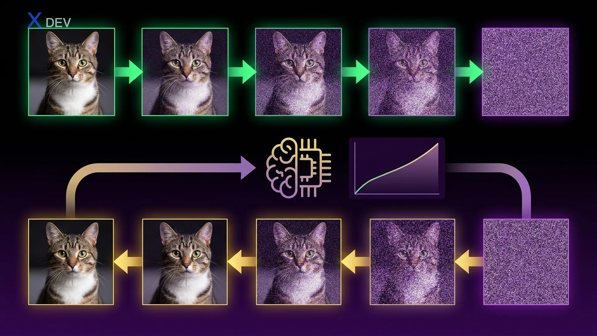
2. 正向擴散過程
2.1 馬可夫鏈公式
正向擴散是在 T 個時間步中逐漸對原始影像 x_0 添加高斯噪聲的過程。這是一條馬可夫鏈——每一步僅依賴於前一步:
q(x_{1:T} | x_0) = ∏_{t=1}^{T} q(x_t | x_{t-1})
在每個時間步 t,我們按照高斯分佈添加噪聲:
q(x_t | x_{t-1}) = N(x_t;  √(1 - β_t) · x_{t-1},  β_t · I)
                         ▲ mean                    ▲ variance
其中 β_t(beta)是變異數排程——一個從 β_1 ≈ 0.0001 逐漸增加到 β_T ≈ 0.02 的小值。它控制每一步添加的噪聲量。
| 符號 | 含義 | 典型值 |
|---|---|---|
| β_t | 時間步 t 的變異數 | 0.0001 → 0.02 |
| α_t = 1 - β_t | 訊號保留比率 | 0.9999 → 0.98 |
| ᾱ_t = ∏_{s=1}^{t} α_s | 累積訊號保留量 | ≈1.0 → ≈0.0 |
| T | 總時間步數 | 1000(原始 DDPM) |
| ε | 標準高斯噪聲 | ε ~ N(0, I) |
2.2 封閉解:直接跳到任意時間步
關鍵洞察:我們不需要逐步執行 T 個正向步驟。得益於高斯分佈的可加性,我們有封閉解可以直接從 x_0 計算 x_t:
q(x_t | x_0) = N(x_t;  √(ᾱ_t) · x_0,  (1 - ᾱ_t) · I)

Where:
  ᾱ_t = α_1 · α_2 · ... · α_t = ∏_{s=1}^{t} (1 - β_s)
這對訓練極為重要——我們可以取樣任意時間步 t,而無需模擬整條鏈。
2.3 重參數化技巧
為了從上述分佈中取樣 x_t 並反向傳播梯度,我們使用重參數化技巧:
x_t = √(ᾱ_t) · x_0  +  √(1 - ᾱ_t) · ε      where ε ~ N(0, I)
      ────────────────   ──────────────────
      signal component    noise component
這個公式表明:在時間步 t,影像 x_t 是原始影像(按 √ᾱ_t 縮放)和純噪聲(按 √(1−ᾱ_t) 縮放)的線性混合。當 t 較小時 → ᾱ_t ≈ 1 → 幾乎全是訊號。當 t 較大時 → ᾱ_t ≈ 0 → 幾乎全是噪聲。
Signal vs Noise across timesteps (T=1000, linear schedule)
══════════════════════════════════════════════════════════

  Signal: √(ᾱ_t)       Noise: √(1-ᾱ_t)
  1.0 ┤████████░░░░░░        0.0 ┤░░░░░░░░████████
      │████████░░░░░░            │░░░░░░░░████████
      │██████░░░░░░░░            │░░░░░░██████████
      │████░░░░░░░░░░            │░░░░████████████
      │██░░░░░░░░░░░░            │░░██████████████
  0.0 ┤░░░░░░░░░░░░░░        1.0 ┤████████████████
      └──────────────            └────────────────
       t=0        t=T             t=0          t=T

  At t ≈ T/2:  signal ≈ noise  (image is half clean, half noise)
  At t = T:    signal ≈ 0      (pure Gaussian noise)
2.4 實作:forward_diffusion()
import torch
import torch.nn as nn
import math

def forward_diffusion(x_0, t, sqrt_alpha_bar, sqrt_one_minus_alpha_bar):
    """
    Apply forward diffusion: x_t = sqrt(alpha_bar_t) * x_0 + sqrt(1 - alpha_bar_t) * eps

    Args:
        x_0: (B, C, H, W) — clean images
        t: (B,) — timestep indices (0-indexed)
        sqrt_alpha_bar: (T,) — precomputed sqrt(ᾱ_t)
        sqrt_one_minus_alpha_bar: (T,) — precomputed sqrt(1 - ᾱ_t)
    Returns:
        x_t: (B, C, H, W) — noisy images at timestep t
        noise: (B, C, H, W) — the noise that was added (needed for loss)
    """
    # Sample Gaussian noise
    noise = torch.randn_like(x_0)

    # Gather coefficients for each sample in batch
    # (B,) -> (B, 1, 1, 1) for broadcasting with (B, C, H, W)
    s_alpha = sqrt_alpha_bar[t].view(-1, 1, 1, 1)
    s_one_minus = sqrt_one_minus_alpha_bar[t].view(-1, 1, 1, 1)

    # Reparameterization: x_t = sqrt(ᾱ_t) * x_0 + sqrt(1-ᾱ_t) * ε
    x_t = s_alpha * x_0 + s_one_minus * noise

    return x_t, noise
考試提示: 注意
.view(-1, 1, 1, 1)——這是在取得純量係數後與 4D 張量進行廣播時的必要模式。忘記重塑形狀會導致維度不匹配。評測中經常考察這一點。
3. 噪聲排程
3.1 線性排程(原始 DDPM)
原始 DDPM 論文使用線性排程:β 在 T = 1000 步內從 β_1 = 0.0001 線性增加到 β_T = 0.02。
def linear_beta_schedule(T, beta_start=1e-4, beta_end=0.02):
    """
    Linear variance schedule: β_t increases linearly from beta_start to beta_end.
    Original DDPM (Ho et al. 2020).
    """
    return torch.linspace(beta_start, beta_end, T)


def precompute_schedule(betas):
    """Precompute all coefficients from beta schedule."""
    alphas = 1.0 - betas                          # α_t = 1 - β_t
    alpha_bar = torch.cumprod(alphas, dim=0)       # ᾱ_t = ∏ α_s
    sqrt_alpha_bar = torch.sqrt(alpha_bar)         # √(ᾱ_t)
    sqrt_one_minus_alpha_bar = torch.sqrt(1.0 - alpha_bar)  # √(1 - ᾱ_t)
    sqrt_alpha = torch.sqrt(alphas)                # √(α_t)  — for reverse step

    return {
        'betas': betas,
        'alphas': alphas,
        'alpha_bar': alpha_bar,
        'sqrt_alpha_bar': sqrt_alpha_bar,
        'sqrt_one_minus_alpha_bar': sqrt_one_minus_alpha_bar,
        'sqrt_alpha': sqrt_alpha,
    }

# Usage
T = 1000
schedule = precompute_schedule(linear_beta_schedule(T))
3.2 餘弦排程(改進版 DDPM)
線性排程的問題:ᾱ_t 在中間區域下降太快 → 影像過早被破壞,導致資訊損失。餘弦排程(Nichol & Dhariwal 2021)透過使用餘弦函數設計 ᾱ_t 來解決此問題——衰減更平滑,對高解析度影像效果尤其更好。
def cosine_beta_schedule(T, s=0.008):
    """
    Cosine variance schedule (Nichol & Dhariwal 2021).
    Designs alpha_bar directly via cosine function, then derives betas.
    The 's' offset prevents beta from being too small near t=0.
    """
    steps = torch.arange(T + 1, dtype=torch.float32)
    # f(t) = cos( (t/T + s) / (1+s) * π/2 )²
    f_t = torch.cos(((steps / T) + s) / (1 + s) * (math.pi / 2)) ** 2
    alpha_bar = f_t / f_t[0]  # normalize so alpha_bar[0] = 1

    # Derive betas from alpha_bar: β_t = 1 - ᾱ_t / ᾱ_{t-1}
    betas = 1 - (alpha_bar[1:] / alpha_bar[:-1])
    betas = torch.clamp(betas, min=1e-5, max=0.999)  # numerical stability

    return betas
| 特性 | 線性排程 | 餘弦排程 |
|---|---|---|
| t=T/2 時的 ᾱ_t | ≈ 0.05(接近 0) | ≈ 0.50(仍有訊號) |
| 訊號破壞 | 快速、激進 | 平滑、漸進 |
| 高解析度影像 | 差(過早失去細節) | 好很多 |
| 原始論文 | DDPM(Ho 2020) | Improved DDPM(Nichol 2021) |
| 用於 Stable Diffusion | 否 | 是(變體) |
| NVIDIA DLI 重點 | 在實驗中實作 | 理解概念、比較差異 |
ᾱ_t Comparison: Linear vs Cosine (T=1000)
══════════════════════════════════════════

  ᾱ_t
  1.0 ┤C C C C L
      │C C C   L
  0.8 ┤  C C    L
      │    C     L
  0.6 ┤    C      L
      │     C      L
  0.4 ┤      C      L
      │       C      L
  0.2 ┤        C      L
      │         C C    L L
  0.0 ┤            C C C L L L L
      └─────────────────────────
       t=0    t=250   t=500  t=750  t=1000

  L = Linear schedule (drops fast mid-range)
  C = Cosine schedule (smooth decay, retains signal longer)

  Key: Cosine retains signal longer → better generation quality
考試提示: 試題會問「為什麼餘弦排程比線性排程更好?」——答案:因為餘弦排程在中間時間步保留訊號更久,避免過早的資訊破壞。使用線性排程時,ᾱ_{T/2} ≈ 0.05 表示在過程進行到一半時已有 95% 的訊號被丟失。
4. 逆向擴散過程
4.1 目標:學習逆向分佈
逆向擴散是相反的過程——從純噪聲 x_T ~ N(0, I) 開始,逐步去噪回到乾淨的影像 x_0。這是需要學習的部分——U-Net 將學習:
p_θ(x_{t-1} | x_t)  =  N(x_{t-1};  μ_θ(x_t, t),  σ²_t · I)
                              ▲ predicted mean      ▲ fixed variance
DDPM 並非直接預測均值 μ,而是採用更優雅的方法:模型預測加入影像的噪聲 ε。從預測的 ε̂ 中,我們推導出均值:
μ_θ(x_t, t) = ────────── · ( x_t  −  ──────────── · ε_θ(x_t, t) )
                  1                      1 - α_t
               ───────                ──────────────
                √(α_t)                 √(1 - ᾱ_t)

Compact form:
                    1              (1 - α_t)
μ_θ(x_t, t) = ───────── · (x_t − ─────────── · ε_θ(x_t, t))
                √(α_t)           √(1 - ᾱ_t)
4.2 取樣演算法
取樣演算法從 x_T 回到 x_0:
Algorithm: DDPM Sampling
════════════════════════
Input: trained model ε_θ, noise schedule {β_t, α_t, ᾱ_t}

1. Sample x_T ~ N(0, I)                  ← start from pure noise
2. For t = T, T-1, ..., 1:
   a. If t > 1: sample z ~ N(0, I)
      Else:     z = 0                     ← no noise at final step
   b. ε̂ = ε_θ(x_t, t)                    ← U-Net predicts noise
   c. μ = (1/√α_t) · (x_t − ((1-α_t)/√(1-ᾱ_t)) · ε̂)
   d. x_{t-1} = μ + σ_t · z              ← denoise one step
      where σ_t = √(β_t)                 ← simplified variance

3. Return x_0
Reverse Process Visualization
═════════════════════════════

  x_T (pure noise)              x_0 (clean image)
  ┌──────────┐                  ┌──────────┐
  │ ·:·:·:·: │   U-Net × T     │ ████████ │
  │ :·:·:·:· │  ──────────►    │ ██    ██ │
  │ ·:·:·:·: │   denoise       │ ██    ██ │
  │ :·:·:·:· │   iteratively   │ ████████ │
  └──────────┘                  └──────────┘

  Step-by-step (T=1000):
  t=1000      t=750       t=500       t=250       t=0
  ┌──────┐   ┌──────┐   ┌──────┐   ┌──────┐   ┌──────┐
  │ ···· │ → │ ░··░ │ → │ ░▓▓░ │ → │ ▓██▓ │ → │ ████ │
  │ ···· │   │ ·░░· │   │ ▓░░▓ │   │ █▓▓█ │   │ █  █ │
  │ ···· │   │ ·░░· │   │ ▓░░▓ │   │ █▓▓█ │   │ █  █ │
  │ ···· │   │ ░··░ │   │ ░▓▓░ │   │ ▓██▓ │   │ ████ │
  └──────┘   └──────┘   └──────┘   └──────┘   └──────┘
  noise only   structure   shape      details    clean!
               emerges     forms      sharpen
4.3 實作:逆向取樣迴圈
@torch.no_grad()
def sample_ddpm(model, shape, schedule, device='cuda'):
    """
    DDPM sampling: generate images from pure noise.

    Args:
        model: trained U-Net noise predictor ε_θ
        shape: (B, C, H, W) — output shape
        schedule: dict with 'betas', 'alphas', 'alpha_bar', etc.
        device: torch device
    Returns:
        x_0: (B, C, H, W) — generated images
    """
    T = len(schedule['betas'])
    betas = schedule['betas'].to(device)
    alphas = schedule['alphas'].to(device)
    alpha_bar = schedule['alpha_bar'].to(device)
    sqrt_alpha = schedule['sqrt_alpha'].to(device)
    sqrt_one_minus_alpha_bar = schedule['sqrt_one_minus_alpha_bar'].to(device)

    # Step 1: Start from pure Gaussian noise
    x_t = torch.randn(shape, device=device)

    # Step 2: Iteratively denoise from t=T-1 down to t=0
    for t in reversed(range(T)):
        t_batch = torch.full((shape[0],), t, device=device, dtype=torch.long)

        # (a) Predict noise using U-Net
        eps_pred = model(x_t, t_batch)

        # (b) Compute predicted mean μ_θ
        #     μ = (1/√α_t) * (x_t - (1-α_t)/√(1-ᾱ_t) * ε̂)
        coeff_xt = 1.0 / sqrt_alpha[t]
        coeff_eps = (1.0 - alphas[t]) / sqrt_one_minus_alpha_bar[t]
        mu = coeff_xt * (x_t - coeff_eps * eps_pred)

        # (c) Add noise (except at t=0)
        if t > 0:
            sigma = torch.sqrt(betas[t])
            z = torch.randn_like(x_t)
            x_t = mu + sigma * z
        else:
            x_t = mu  # final step: no noise added

    return x_t
考試提示: 取樣迴圈中最常見的兩個錯誤:(1) 忘記
@torch.no_grad()→ 使用 3-4 倍的 VRAM,OOM 崩潰。(2) 在步驟 t=0 時添加噪聲 → 輸出影像仍然帶有噪聲。務必在添加 z 之前檢查if t > 0。
5. 訓練目標:簡化 ELBO 損失
5.1 從 ELBO 到簡化損失
理論上,DDPM 最佳化的是對數似然的變分下界(ELBO)。但 Ho et al. 發現簡化損失在實務上效果更好:
Full ELBO Loss (theoretical):
L_vlb = L_0 + L_1 + ... + L_{T-1} + L_T
      = ∑_t KL(q(x_{t-1}|x_t,x_0) || p_θ(x_{t-1}|x_t))

Simplified Loss (practical — DDPM paper):
L_simple = E_{t ~ U{1,T}, x_0, ε} [ || ε − ε_θ(x_t, t) ||² ]

Meaning:
  - Sample a random timestep t
  - Create x_t from x_0 via forward diffusion
  - U-Net predicts noise ε̂ = ε_θ(x_t, t)
  - Loss = MSE between actual noise (ε) and predicted noise (ε̂)
這正是為什麼你需要從 forward_diffusion() 回傳 noise 的原因——它作為訓練的真實標籤。
5.2 訓練演算法
Algorithm: DDPM Training
════════════════════════
Repeat until convergence:
  1. Sample x_0 ~ q(x_0)              ← batch from dataset
  2. Sample t ~ Uniform({1, ..., T})   ← random timestep per sample
  3. Sample ε ~ N(0, I)               ← target noise
  4. Compute x_t = √(ᾱ_t)·x_0 + √(1−ᾱ_t)·ε    ← forward diffusion
  5. Compute ε̂ = ε_θ(x_t, t)          ← U-Net predicts noise
  6. Loss = MSE(ε, ε̂)                 ← compare real vs predicted noise
  7. Backprop & update θ
5.3 實作:完整訓練迴圈
def train_ddpm(model, dataloader, schedule, epochs=100, lr=2e-4, device='cuda'):
    """
    Full DDPM training loop.

    Args:
        model: U-Net noise predictor
        dataloader: yields (images, labels) batches
        schedule: precomputed noise schedule dict
        epochs: number of training epochs
        lr: learning rate
        device: torch device
    """
    optimizer = torch.optim.Adam(model.parameters(), lr=lr)
    loss_fn = nn.MSELoss()
    T = len(schedule['betas'])

    sqrt_alpha_bar = schedule['sqrt_alpha_bar'].to(device)
    sqrt_one_minus_alpha_bar = schedule['sqrt_one_minus_alpha_bar'].to(device)

    model.train()
    for epoch in range(epochs):
        epoch_loss = 0.0
        for batch_idx, (x_0, _) in enumerate(dataloader):
            x_0 = x_0.to(device)
            B = x_0.shape[0]

            # Step 2: Sample random timesteps
            t = torch.randint(0, T, (B,), device=device)

            # Steps 3-4: Forward diffusion (sample noise + compute x_t)
            x_t, noise = forward_diffusion(
                x_0, t, sqrt_alpha_bar, sqrt_one_minus_alpha_bar
            )

            # Step 5: Predict noise
            noise_pred = model(x_t, t)

            # Step 6: Compute loss
            loss = loss_fn(noise_pred, noise)

            # Step 7: Backprop
            optimizer.zero_grad()
            loss.backward()
            optimizer.step()

            epoch_loss += loss.item()

        avg_loss = epoch_loss / len(dataloader)
        if (epoch + 1) % 10 == 0:
            print(f"Epoch {epoch+1}/{epochs}, Loss: {avg_loss:.4f}")
| 訓練元件 | 角色 | 對應程式碼 |
|---|---|---|
| 來自資料集的 x_0 | 乾淨影像輸入 | x_0 = batch[0].to(device) |
| t ~ Uniform | 隨機時間步 | torch.randint(0, T, (B,)) |
| ε ~ N(0,I) | 目標噪聲 | torch.randn_like(x_0) |
| 透過重參數化的 x_t | 含噪影像 | forward_diffusion(...) |
| ε_θ(x_t, t) | U-Net 預測 | model(x_t, t) |
| MSE(ε, ε̂) | 簡化損失 | nn.MSELoss()(pred, target) |
考試提示: 在評測中,你需要從頭撰寫訓練迴圈。步驟順序至關重要:正向擴散 → 預測 → 損失 → 反向傳播。如果將
optimizer.zero_grad()放在錯誤位置或忘記loss.backward(),模型將無法學習——你將失去分數。
6. 無分類器擴散引導(CFG)
6.1 條件生成與 CFG
原始 DDPM 無條件地生成影像。若要根據條件(類別標籤、文字提示)生成影像,我們需要條件生成。Classifier-Free Guidance(CFG)是最優雅的方法:
Classifier-Free Guidance
═════════════════════════

  Training: Model receives condition c, but randomly drops c → ∅ with probability p_uncond
  ┌──────────────────────────────────────┐
  │  if random() < p_uncond (e.g. 0.1): │
  │      c = ∅  (null / empty)           │    ← 10% unconditional
  │  ε̂ = ε_θ(x_t, t, c)                 │
  └──────────────────────────────────────┘

  Inference: Combine conditional & unconditional predictions
  ┌──────────────────────────────────────────────────────────────┐
  │  ε̂_uncond = ε_θ(x_t, t, ∅)           ← unconditional pred  │
  │  ε̂_cond   = ε_θ(x_t, t, c)           ← conditional pred    │
  │                                                              │
  │  ε̂_guided = ε̂_uncond + w · (ε̂_cond − ε̂_uncond)             │
  │              ▲                 ▲ guidance direction           │
  │              baseline          amplified by scale w           │
  └──────────────────────────────────────────────────────────────┘

  w = guidance scale:
    w = 1.0  → standard conditional (no guidance)
    w = 7.5  → typical value (Stable Diffusion default)
    w = 20   → very strong guidance → faithful but less diverse
    w = 0.0  → purely unconditional
6.2 引導強度的權衡
| 引導強度 w | 品質 | 多樣性 | 條件忠實度 | 使用場景 |
|---|---|---|---|---|
| 0.0 | 低 | 非常高 | 無(無條件) | 探索 |
| 1.0 | 中等 | 高 | 標準 | 無引導 |
| 3.0 – 5.0 | 良好 | 中等 | 良好 | 平衡生成 |
| 7.0 – 8.5 | 非常好 | 較低 | 非常好 | Stable Diffusion 預設值 |
| 15.0 – 20.0 | 過度飽和 | 非常低 | 過度 | 藝術風格化 |
6.3 實作:CFG 訓練與取樣
def train_ddpm_cfg(model, dataloader, schedule, epochs=100,
                   lr=2e-4, p_uncond=0.1, num_classes=10, device='cuda'):
    """
    DDPM training with Classifier-Free Guidance.
    Model takes (x_t, t, class_label) as input.
    During training, randomly replace class_label with null_class.
    """
    optimizer = torch.optim.Adam(model.parameters(), lr=lr)
    loss_fn = nn.MSELoss()
    T = len(schedule['betas'])
    null_class = num_classes  # use num_classes as "no class" token

    sqrt_ab = schedule['sqrt_alpha_bar'].to(device)
    sqrt_omab = schedule['sqrt_one_minus_alpha_bar'].to(device)

    model.train()
    for epoch in range(epochs):
        for x_0, labels in dataloader:
            x_0, labels = x_0.to(device), labels.to(device)
            B = x_0.shape[0]

            # Random timestep
            t = torch.randint(0, T, (B,), device=device)

            # CFG: randomly drop condition
            mask = torch.rand(B, device=device) < p_uncond
            labels_cfg = labels.clone()
            labels_cfg[mask] = null_class  # replace with null token

            # Forward diffusion
            x_t, noise = forward_diffusion(x_0, t, sqrt_ab, sqrt_omab)

            # Predict noise (conditioned on possibly-null label)
            noise_pred = model(x_t, t, labels_cfg)

            # Loss
            loss = loss_fn(noise_pred, noise)
            optimizer.zero_grad()
            loss.backward()
            optimizer.step()


@torch.no_grad()
def sample_ddpm_cfg(model, shape, schedule, class_label, guidance_scale=7.5,
                    num_classes=10, device='cuda'):
    """
    DDPM sampling with Classifier-Free Guidance.

    ε̂_guided = ε̂_uncond + w * (ε̂_cond - ε̂_uncond)

    Args:
        class_label: (B,) — target class for each sample
        guidance_scale: w — higher = more faithful to condition
    """
    T = len(schedule['betas'])
    betas = schedule['betas'].to(device)
    alphas = schedule['alphas'].to(device)
    alpha_bar = schedule['alpha_bar'].to(device)
    sqrt_alpha = schedule['sqrt_alpha'].to(device)
    sqrt_omab = schedule['sqrt_one_minus_alpha_bar'].to(device)
    null_class = num_classes

    x_t = torch.randn(shape, device=device)
    class_label = class_label.to(device)
    null_label = torch.full_like(class_label, null_class)

    for t in reversed(range(T)):
        t_batch = torch.full((shape[0],), t, device=device, dtype=torch.long)

        # Two forward passes: conditional + unconditional
        eps_cond = model(x_t, t_batch, class_label)    # ε_θ(x_t, t, c)
        eps_uncond = model(x_t, t_batch, null_label)   # ε_θ(x_t, t, ∅)

        # CFG formula
        eps_guided = eps_uncond + guidance_scale * (eps_cond - eps_uncond)

        # Compute mean
        coeff_xt = 1.0 / sqrt_alpha[t]
        coeff_eps = (1.0 - alphas[t]) / sqrt_omab[t]
        mu = coeff_xt * (x_t - coeff_eps * eps_guided)

        # Denoise step
        if t > 0:
            sigma = torch.sqrt(betas[t])
            x_t = mu + sigma * torch.randn_like(x_t)
        else:
            x_t = mu

    return x_t
考試提示: CFG 每個取樣步驟需要兩次前向傳遞——一次有條件、一次無條件。這就是為什麼使用 CFG 取樣速度慢兩倍。在 DLI 實驗中,如果你只執行一次前向傳遞,引導將不會生效——輸出結果將與無條件相同。
7. 速查表:DDPM 公式總結
| 公式 | 含義 | 使用場景 |
|---|---|---|
| x_t = √ᾱ_t · x_0 + √(1−ᾱ_t) · ε | 正向擴散(封閉解) | 訓練:從 x_0 建立 x_t |
| ε̂ = ε_θ(x_t, t) | U-Net 預測噪聲 | 訓練:輸出 | 取樣:去噪 |
| L = MSE(ε, ε̂) | 簡化 ELBO 損失 | 訓練:計算損失 |
| μ = (1/√α_t)(x_t − (1−α_t)/√(1−ᾱ_t) · ε̂) | 逆向步驟的預測均值 | 取樣:計算 μ_θ |
| x_{t−1} = μ + √β_t · z | 取樣步驟(t=0 時 z=0) | 取樣:去噪一步 |
| ε̂ = ε̂_∅ + w(ε̂_c − ε̂_∅) | CFG 引導公式 | 條件取樣 |
DDPM Pipeline Summary
═════════════════════

  ┌─────────────────────────────────────────────────────────┐
  │                      TRAINING                           │
  │                                                         │
  │  x_0 ──[forward_diffusion]──► x_t ──[U-Net]──► ε̂      │
  │   │         ↑                                    │      │
  │   └─── t,ε (random) ───────────────── MSE(ε, ε̂) │      │
  │                                         │               │
  │                                    backprop             │
  └─────────────────────────────────────────────────────────┘

  ┌─────────────────────────────────────────────────────────┐
  │                     SAMPLING                            │
  │                                                         │
  │  x_T ──► [U-Net] ──► ε̂ ──► μ_θ ──► x_{T-1}           │
  │                                       │                 │
  │         [U-Net] ──► ε̂ ──► μ_θ ──► x_{T-2}             │
  │                                       │                 │
  │         ...repeat T times...          │                 │
  │                                       ▼                 │
  │                                      x_0 (generated!)  │
  └─────────────────────────────────────────────────────────┘

  ┌─────────────────────────────────────────────────────────┐
  │                   CFG SAMPLING                          │
  │                                                         │
  │  At each step t:                                        │
  │    ε̂_∅ = UNet(x_t, t, null)      ← unconditional      │
  │    ε̂_c = UNet(x_t, t, class)     ← conditional        │
  │    ε̂ = ε̂_∅ + w · (ε̂_c − ε̂_∅)   ← guided prediction  │
  │    x_{t-1} = denoise(x_t, ε̂)                          │
  └─────────────────────────────────────────────────────────┘
8. 練習題
5 道程式題——嘗試自行實作後再查看答案。
Q1:實作 forward_diffusion(x_0, t, noise_schedule) → x_t, noise
撰寫 forward_diffusion 函式,接收一批影像 x_0、一個時間步張量 t,以及一個包含預計算係數的字典 noise_schedule。回傳 x_t 和使用的噪聲 ε。
def forward_diffusion(x_0, t, noise_schedule):
    """
    Args:
        x_0: (B, C, H, W) — clean images, normalized to [-1, 1]
        t: (B,) — integer timestep indices
        noise_schedule: dict with keys:
            'sqrt_alpha_bar': (T,) tensor
            'sqrt_one_minus_alpha_bar': (T,) tensor
    Returns:
        x_t: (B, C, H, W) — noisy images
        noise: (B, C, H, W) — the Gaussian noise added
    """
    # TODO: Implement forward diffusion using reparameterization trick
    pass
顯示答案 Q1
def forward_diffusion(x_0, t, noise_schedule):
    sqrt_alpha_bar = noise_schedule['sqrt_alpha_bar']
    sqrt_one_minus_alpha_bar = noise_schedule['sqrt_one_minus_alpha_bar']

    # Sample noise ε ~ N(0, I)
    noise = torch.randn_like(x_0)

    # Gather coefficients for batch and reshape for broadcasting
    # (B,) → (B, 1, 1, 1)
    s_ab = sqrt_alpha_bar[t].view(-1, 1, 1, 1)
    s_omab = sqrt_one_minus_alpha_bar[t].view(-1, 1, 1, 1)

    # Reparameterization trick:
    # x_t = √(ᾱ_t) * x_0 + √(1 - ᾱ_t) * ε
    x_t = s_ab * x_0 + s_omab * noise

    return x_t, noise
說明:三個關鍵步驟:(1) 使用 torch.randn_like 取樣與 x_0 相同形狀的噪聲,(2) 按索引 t 取得係數後使用 .view(-1, 1, 1, 1) 重塑以進行 4D 廣播,(3) 套用重參數化技巧。注意我們必須同時回傳噪聲,因為訓練迴圈需要它作為 MSE 損失的目標。
Q2:實作逆向擴散取樣迴圈
撰寫 sample_ddpm 函式,透過迭代逆向擴散步驟從純噪聲生成新影像。模型已經訓練完成。
@torch.no_grad()
def sample_ddpm(model, n_samples, img_channels, img_size, schedule, device):
    """
    Args:
        model: trained U-Net, expects (x_t, t_batch) → predicted noise
        n_samples: int — number of images to generate
        img_channels: int — e.g., 1 for MNIST
        img_size: int — e.g., 28
        schedule: dict with 'betas', 'alphas', 'alpha_bar',
                  'sqrt_alpha', 'sqrt_one_minus_alpha_bar'
    Returns:
        images: (n_samples, C, H, W) — generated images
    """
    # TODO: Implement the full DDPM sampling algorithm
    pass
顯示答案 Q2
@torch.no_grad()
def sample_ddpm(model, n_samples, img_channels, img_size, schedule, device):
    T = len(schedule['betas'])
    betas = schedule['betas'].to(device)
    alphas = schedule['alphas'].to(device)
    sqrt_alpha = schedule['sqrt_alpha'].to(device)
    sqrt_omab = schedule['sqrt_one_minus_alpha_bar'].to(device)

    shape = (n_samples, img_channels, img_size, img_size)

    # Start from pure noise x_T ~ N(0, I)
    x_t = torch.randn(shape, device=device)

    for t in reversed(range(T)):
        t_batch = torch.full((n_samples,), t, device=device, dtype=torch.long)

        # U-Net predicts noise
        eps_pred = model(x_t, t_batch)

        # Compute predicted mean:
        # μ_θ = (1/√α_t) * (x_t − ((1−α_t) / √(1−ᾱ_t)) * ε̂)
        coeff_xt = 1.0 / sqrt_alpha[t]
        coeff_eps = (1.0 - alphas[t]) / sqrt_omab[t]
        mu = coeff_xt * (x_t - coeff_eps * eps_pred)

        # Sample x_{t-1}: add noise for t > 0, otherwise return mean
        if t > 0:
            sigma = torch.sqrt(betas[t])
            z = torch.randn_like(x_t)
            x_t = mu + sigma * z
        else:
            x_t = mu

    return x_t
說明:取樣迴圈從 t=T-1 逆向執行到 t=0。每一步:(1) U-Net 預測噪聲 ε̂,(2) 使用 DDPM 公式計算均值 μ_θ,(3) 如果 t > 0 則添加噪聲 z(隨機取樣)。關鍵:使用 @torch.no_grad() 避免在 1000 步中累積梯度——否則會導致 OOM。步驟 t=0 不添加噪聲,因為這是最終輸出。
Q3:除錯——模型輸出黑色影像
一位學生實作了逆向取樣,但結果總是黑色影像(接近 0)。找出以下程式碼中的錯誤:
@torch.no_grad()
def buggy_sample(model, shape, schedule, device):
    T = len(schedule['betas'])
    betas = schedule['betas'].to(device)
    alphas = schedule['alphas'].to(device)
    sqrt_alpha = schedule['sqrt_alpha'].to(device)
    sqrt_omab = schedule['sqrt_one_minus_alpha_bar'].to(device)

    x_t = torch.randn(shape, device=device)

    for t in reversed(range(T)):
        t_batch = torch.full((shape[0],), t, device=device, dtype=torch.long)
        eps_pred = model(x_t, t_batch)

        # BUG IS HERE — find it!
        coeff_xt = 1.0 / sqrt_alpha[t]
        coeff_eps = (1.0 - alphas[t]) / sqrt_omab[t]
        mu = coeff_xt * (x_t + coeff_eps * eps_pred)  # line A

        if t > 0:
            sigma = torch.sqrt(betas[t])
            x_t = mu + sigma * torch.randn_like(x_t)
        else:
            x_t = mu

    return x_t
顯示答案 Q3
錯誤: 計算 μ 的那一行在 coeff_eps * eps_pred 前使用了 + 而非 −。
# BUG (line A):
mu = coeff_xt * (x_t + coeff_eps * eps_pred)   # ← WRONG: + instead of -

# FIX:
mu = coeff_xt * (x_t - coeff_eps * eps_pred)   # ← CORRECT: subtract noise
說明:DDPM 逆向均值公式為 μ = (1/√α_t)(x_t − ((1−α_t)/√(1−ᾱ_t)) · ε̂)。減號是「去噪」的精髓——我們減去預測的噪聲。使用加號時,我們實際上是添加更多噪聲而非移除噪聲 → 經過 1000 步後,影像被中和(在 0 附近震盪)→ 輸出接近 0(黑色)。這是一個微妙的錯誤,因為程式碼仍然正常執行、輸出形狀也正確——只有數值是錯的。
Q4:實作帶引導強度的 CFG 取樣
模型已使用條件丟棄進行訓練。撰寫一個帶有 Classifier-Free Guidance 的取樣函式。
@torch.no_grad()
def sample_cfg(model, shape, schedule, class_labels, guidance_scale,
               num_classes, device):
    """
    Args:
        model: U-Net with signature model(x_t, t, class_label) → noise
        shape: (B, C, H, W)
        class_labels: (B,) — target class indices
        guidance_scale: float w — e.g. 7.5
        num_classes: int — total classes (null_class = num_classes)
    Returns:
        images: (B, C, H, W)
    """
    # TODO: Implement CFG sampling
    # Hint: two forward passes per step — conditional & unconditional
    pass
顯示答案 Q4
@torch.no_grad()
def sample_cfg(model, shape, schedule, class_labels, guidance_scale,
               num_classes, device):
    T = len(schedule['betas'])
    betas = schedule['betas'].to(device)
    alphas = schedule['alphas'].to(device)
    sqrt_alpha = schedule['sqrt_alpha'].to(device)
    sqrt_omab = schedule['sqrt_one_minus_alpha_bar'].to(device)
    null_class = num_classes

    x_t = torch.randn(shape, device=device)
    class_labels = class_labels.to(device)
    null_labels = torch.full_like(class_labels, null_class)

    for t in reversed(range(T)):
        t_batch = torch.full((shape[0],), t, device=device, dtype=torch.long)

        # Two forward passes
        eps_uncond = model(x_t, t_batch, null_labels)   # ε_θ(x_t, t, ∅)
        eps_cond = model(x_t, t_batch, class_labels)    # ε_θ(x_t, t, c)

        # CFG: ε̂ = ε_uncond + w * (ε_cond - ε_uncond)
        eps_guided = eps_uncond + guidance_scale * (eps_cond - eps_uncond)

        # Reverse step with guided noise prediction
        coeff_xt = 1.0 / sqrt_alpha[t]
        coeff_eps = (1.0 - alphas[t]) / sqrt_omab[t]
        mu = coeff_xt * (x_t - coeff_eps * eps_guided)

        if t > 0:
            sigma = torch.sqrt(betas[t])
            x_t = mu + sigma * torch.randn_like(x_t)
        else:
            x_t = mu

    return x_t
說明:CFG 取樣與標準取樣的不同之處在於每一步需要執行兩次 U-Net 前向傳遞:(1) 使用 null_class 的無條件傳遞,(2) 使用實際類別的有條件傳遞。然後組合:ε̂ = ε̂_∅ + w·(ε̂_c − ε̂_∅)。當 w=1.0 → 標準條件生成(無引導)。當 w>1.0 → 放大有條件與無條件之間的差異 → 影像更銳利但多樣性降低。null_class 通常 = num_classes(一個超出實際類別的索引)。
Q5:比較線性排程與餘弦排程——ᾱ_t 在何時降到 0.01 以下?
撰寫程式碼計算並比較:當 T=1000 時,每種排程的 ᾱ_t 在哪個時間步降到 0.01 以下?這對生成品質意味著什麼?
def compare_schedules(T=1000):
    """
    Compute alpha_bar for both linear and cosine schedules.
    Find the timestep where alpha_bar drops below 0.01 for each.
    Print comparison results.
    """
    # TODO: implement using linear_beta_schedule() and cosine_beta_schedule()
    pass
顯示答案 Q5
import torch
import math

def linear_beta_schedule(T, beta_start=1e-4, beta_end=0.02):
    return torch.linspace(beta_start, beta_end, T)

def cosine_beta_schedule(T, s=0.008):
    steps = torch.arange(T + 1, dtype=torch.float32)
    f_t = torch.cos(((steps / T) + s) / (1 + s) * (math.pi / 2)) ** 2
    alpha_bar = f_t / f_t[0]
    betas = 1 - (alpha_bar[1:] / alpha_bar[:-1])
    return torch.clamp(betas, min=1e-5, max=0.999)

def compare_schedules(T=1000):
    # Linear schedule
    betas_lin = linear_beta_schedule(T)
    alphas_lin = 1.0 - betas_lin
    alpha_bar_lin = torch.cumprod(alphas_lin, dim=0)

    # Cosine schedule
    betas_cos = cosine_beta_schedule(T)
    alphas_cos = 1.0 - betas_cos
    alpha_bar_cos = torch.cumprod(alphas_cos, dim=0)

    # Find where alpha_bar < 0.01
    threshold = 0.01
    t_lin = (alpha_bar_lin < threshold).nonzero(as_tuple=True)[0][0].item()
    t_cos = (alpha_bar_cos < threshold).nonzero(as_tuple=True)[0][0].item()

    print(f"Linear schedule: ᾱ_t < {threshold} at t = {t_lin}")
    print(f"  ᾱ at t=250: {alpha_bar_lin[250]:.4f}")
    print(f"  ᾱ at t=500: {alpha_bar_lin[500]:.4f}")
    print(f"  ᾱ at t=750: {alpha_bar_lin[750]:.6f}")
    print()
    print(f"Cosine schedule: ᾱ_t < {threshold} at t = {t_cos}")
    print(f"  ᾱ at t=250: {alpha_bar_cos[250]:.4f}")
    print(f"  ᾱ at t=500: {alpha_bar_cos[500]:.4f}")
    print(f"  ᾱ at t=750: {alpha_bar_cos[750]:.4f}")
    print()
    print(f"Difference: cosine retains signal for {t_cos - t_lin} more timesteps")

compare_schedules()
# Output (approximate):
# Linear schedule: ᾱ_t < 0.01 at t ≈ 650
#   ᾱ at t=250: 0.6766
#   ᾱ at t=500: 0.0473
#   ᾱ at t=750: 0.000014
#
# Cosine schedule: ᾱ_t < 0.01 at t ≈ 940
#   ᾱ at t=250: 0.8536
#   ᾱ at t=500: 0.5000
#   ᾱ at t=750: 0.1464
#
# Difference: cosine retains signal for ~290 more timesteps
說明:線性排程過早破壞訊號——ᾱ_t < 0.01 大約在 t≈650,意味著鏈的最後 35% 幾乎是無用的(噪聲實際上已是純噪聲)。餘弦排程將 ᾱ_t > 0.01 維持到 t≈940,更有效率地利用所有 T 個步驟。特別注意:在 t=500(鏈的中點),線性排程的 ᾱ≈0.05(5% 訊號),而餘弦排程仍有 ᾱ≈0.50(50% 訊號)。這解釋了為什麼餘弦排程產生更好的生成品質——模型從更多時間步獲得有用的梯度,不會在純噪聲區域浪費計算。
考試提示: 在 DLI 評測中,關於噪聲排程的問題通常要求你解釋為什麼某種排程更好。關鍵洞察:好的排程應將訊號破壞均勻分佈在所有時間步上——不會太快(線性)也不會太慢。餘弦排程透過直接設計 ᾱ_t 而非 β_t 來達成此目標。