1. 前言:從類別標籤到文字提示
在上一課中,你實作了使用類別標籤(數字0–9)的無分類器引導(CFG)。但Stable Diffusion不使用類別標籤——它使用自由格式的文字提示。那麼,我們如何將「a photo of a cat」轉換為U-Net能夠理解的張量呢?
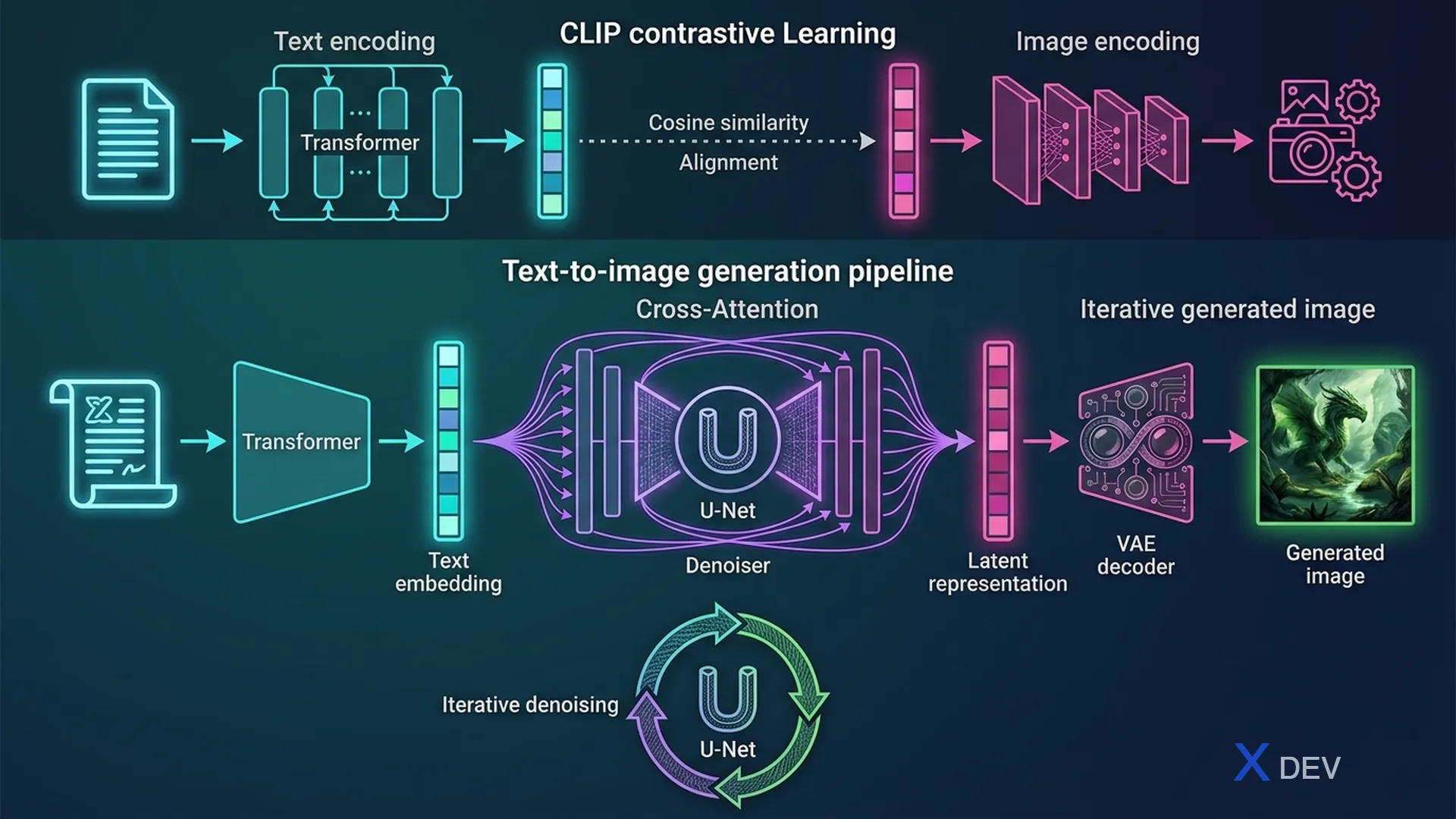
答案在於CLIP(Contrastive Language-Image Pretraining)——OpenAI於2021年推出的語言與圖像之間的橋樑模型。這是Diffusion Models部分的最後一課,結合你所學到的所有知識來建構一個完整的文字到圖像管線。
考試提示: DLI考核S-FX-14要求你將U-Net、DDPM、CFG和文字條件結合成完整的管線。這一課是「大綜合」——如果你徹底理解第3–4課的每個組件,並在第5課中將它們串連起來,你將能更快地完成考核。
Roadmap: Class Label → Text Prompt Conditioning
════════════════════════════════════════════════

  Lesson 3: U-Net backbone          → Denoiser architecture
  Lesson 4: DDPM + CFG              → Training & sampling with class labels
  Lesson 5: CLIP + Cross-Attention  → Text-to-image pipeline ← YOU ARE HERE
        │
        ▼
  ┌──────────────────────────────────────────────────────────┐
  │  "a sunset over mountains"                               │
  │         │                                                │
  │         ▼                                                │
  │   ┌──────────┐   ┌──────────────────┐   ┌──────────┐   │
  │   │   CLIP   │──►│  Cross-Attention  │──►│  U-Net   │   │
  │   │ Encoder  │   │  (K, V from text) │   │ Denoise  │   │
  │   └──────────┘   └──────────────────┘   └──────────┘   │
  │                                              │          │
  │                                              ▼          │
  │                                        [ 🖼️ Image ]     │
  └──────────────────────────────────────────────────────────┘
2. CLIP — 對比語言-圖像預訓練
2.1 雙編碼器架構
CLIP由兩個編碼器組成,同時在來自網際網路的4億(文字、圖像)配對上進行訓練:
- 文字編碼器:Transformer(類似GPT)——輸入文字 → 輸出嵌入向量(512維或768維)
- 圖像編碼器:ViT(Vision Transformer)或ResNet——輸入圖像 → 輸出相同維度的嵌入
關鍵在於:兩個編碼器都在同一個向量空間中輸出嵌入。這使得可以使用餘弦相似度直接比較文字和圖像。
CLIP Architecture — Dual Encoder
═════════════════════════════════

  TEXT BRANCH                          IMAGE BRANCH
  ───────────                          ────────────

  "a photo of    ┌───────────────┐     ┌─────┐   ┌───────────────┐
   a cat"    ──► │ Text Encoder  │     │ 🖼️  │──►│ Image Encoder │
                 │ (Transformer) │     │     │   │ (ViT / ResNet)│
                 └───────┬───────┘     └─────┘   └───────┬───────┘
                         │                                │
                         ▼                                ▼
                  ┌──────────────┐                 ┌──────────────┐
                  │ Text Embed.  │                 │ Image Embed. │
                  │ (768-dim)    │                 │ (768-dim)    │
                  └──────┬───────┘                 └──────┬───────┘
                         │                                │
                         └────────────┬───────────────────┘
                                      │
                                      ▼
                              ┌───────────────┐
                              │    Cosine      │
                              │  Similarity    │
                              │  sim(t, i)     │
                              └───────────────┘

  Training (400M image-text pairs):
  ┌──────────────────────────────────────────────────────┐
  │  Maximize sim(text_i, image_i)    ← matched pairs    │
  │  Minimize sim(text_i, image_j)    ← non-matched      │
  └──────────────────────────────────────────────────────┘
2.2 對比損失
CLIP使用NxN相似度矩陣上的對稱交叉熵損失。給定一個包含N個(文字、圖像)配對的批次:
Contrastive Loss — Similarity Matrix
═════════════════════════════════════

  Batch N = 4 pairs (text, image):

              image_0   image_1   image_2   image_3
            ┌─────────┬─────────┬─────────┬─────────┐
  text_0    │  0.95 ✓ │  0.12   │  0.08   │  0.03   │
            ├─────────┼─────────┼─────────┼─────────┤
  text_1    │  0.10   │  0.91 ✓ │  0.15   │  0.07   │
            ├─────────┼─────────┼─────────┼─────────┤
  text_2    │  0.05   │  0.11   │  0.93 ✓ │  0.09   │
            ├─────────┼─────────┼─────────┼─────────┤
  text_3    │  0.08   │  0.06   │  0.12   │  0.89 ✓ │
            └─────────┴─────────┴─────────┴─────────┘

  Goal: diagonal (✓) → high, rest → low

  Loss = (CE_rows + CE_cols) / 2
       = cross_entropy(logits, labels) for both dimensions

  logits = temperature * text_embeds @ image_embeds.T
  labels = [0, 1, 2, ..., N-1]   ← identity matching
溫度參數(可學習,初始值約0.07)控制分佈的銳度。溫度越低 → 正負配對之間的區別越明顯。
| 組件 | 細節 | 在CLIP中 |
|---|---|---|
| 文字編碼器 | 12層Transformer,BPE分詞器 | 最多77個token,輸出CLS嵌入 |
| 圖像編碼器 | ViT-B/32或ViT-L/14 | 將圖像切分為patch,輸出CLS |
| 嵌入維度 | 512(ViT-B/32)或768(ViT-L/14) | 文字與圖像共享空間 |
| 訓練資料 | 4億圖文配對(WIT資料集) | 從網際網路爬取 |
| 損失函數 | 對稱交叉熵 | InfoNCE / NT-Xent變體 |
| 溫度 | 可學習純量τ | 初始值≈0.07,訓練中學習 |
考試提示: CLIP不會生成圖像——它只是將文字和圖像編碼到共享空間中。在文字到圖像管線中,我們只使用CLIP的文字編碼器來為U-Net建立條件訊號。圖像編碼器在生成過程中不會被使用。
3. 在程式碼中使用CLIP編碼
3.1 載入CLIP並編碼文字
import torch
import clip
from PIL import Image

# Load pretrained CLIP model
device = "cuda" if torch.cuda.is_available() else "cpu"
model, preprocess = clip.load("ViT-B/32", device=device)

# ── Encode text ──
text_prompts = ["a photo of a cat", "a sunset over mountains", "a red car"]
text_tokens = clip.tokenize(text_prompts).to(device)  # (3, 77) — padded to 77 tokens

with torch.no_grad():
    text_embeddings = model.encode_text(text_tokens)  # (3, 512)
    text_embeddings = text_embeddings / text_embeddings.norm(dim=-1, keepdim=True)  # L2 normalize

print(f"Text embeddings shape: {text_embeddings.shape}")  # (3, 512)
3.2 編碼圖像並計算相似度
# ── Encode images ──
images = [preprocess(Image.open(f"img_{i}.jpg")).unsqueeze(0) for i in range(3)]
image_batch = torch.cat(images).to(device)  # (3, 3, 224, 224)

with torch.no_grad():
    image_embeddings = model.encode_image(image_batch)   # (3, 512)
    image_embeddings = image_embeddings / image_embeddings.norm(dim=-1, keepdim=True)

# ── Cosine similarity ──
similarity = text_embeddings @ image_embeddings.T  # (3, 3)
print(similarity)
# tensor([[ 0.31,  0.05,  0.02],    ← "cat" matches image_0
#         [ 0.04,  0.28,  0.06],    ← "sunset" matches image_1
#         [ 0.03,  0.07,  0.26]])   ← "red car" matches image_2
結果:內容匹配的文字和圖像具有最高的相似度。這就是共享嵌入空間的強大之處——你可以用文字搜尋圖像,反之亦然。
3.3 用於Diffusion Models的CLIP:序列嵌入
重要:Stable Diffusion不使用CLS嵌入(單一向量)。相反,它使用CLIP文字編碼器的token嵌入序列——即投影層之前的輸出:
CLS Embedding vs Sequence Embeddings
═════════════════════════════════════

  Text: "a photo of a cat"
  Tokenized: [SOS, "a", "photo", "of", "a", "cat", EOS, PAD, PAD, ...]

  CLIP Text Encoder output:
  ┌──────────────────────────────────────────────┐
  │  token_0 (SOS)  → [0.12, -0.34, 0.56, ...]  │
  │  token_1 ("a")  → [0.08, -0.21, 0.43, ...]  │
  │  token_2 ("photo") → [...]                   │
  │  token_3 ("of") → [...]                      │
  │  token_4 ("a")  → [...]                      │
  │  token_5 ("cat")→ [0.91, 0.15, -0.33, ...]  │  ← semantic info
  │  token_6 (EOS)  → [0.67, 0.42, -0.18, ...]  │  ← CLS (used by CLIP)
  │  ...                                         │
  │  token_76 (PAD) → [0.00, 0.00, 0.00, ...]   │
  └──────────────────────────────────────────────┘

  Stable Diffusion uses: ALL 77 token embeddings → (1, 77, 768)
  CLIP zero-shot uses:   ONLY the EOS token embedding → (1, 768)
| 使用場景 | 輸出 | 形狀 | 原因 |
|---|---|---|---|
| CLIP分類 | CLS / EOS token | (B, 768) | 全域相似度比較 |
| Stable Diffusion | 完整token序列 | (B, 77, 768) | 交叉注意力需要逐token資訊 |
考試提示: 如果題目問「文字條件輸入到U-Net的形狀是什麼?」,答案是(batch, 77, 768)——不是(batch, 768)。交叉注意力需要一個序列,而不是單一向量。
4. 交叉注意力:將文字嵌入注入U-Net
4.1 交叉注意力機制
在第3課中,U-Net使用自注意力——Q、K、V全部來自圖像特徵。交叉注意力改變了K和V的來源:
Self-Attention vs Cross-Attention
═════════════════════════════════

  SELF-ATTENTION (in U-Net):
  ───────────────────────────────
  Q = W_q · image_features    ← from image
  K = W_k · image_features    ← from image
  V = W_v · image_features    ← from image

  Attention = softmax(Q · K^T / √d) · V

  CROSS-ATTENTION (text → image):
  ────────────────────────────────
  Q = W_q · image_features    ← from image (queries)
  K = W_k · text_embeddings   ← from CLIP text (keys)
  V = W_v · text_embeddings   ← from CLIP text (values)

  Attention = softmax(Q_image · K_text^T / √d) · V_text

  ┌──────────────────────────────────────────────────┐
  │  Q shape: (B, H*W, d_model)    ← spatial pixels  │
  │  K shape: (B, 77, d_model)     ← text tokens      │
  │  V shape: (B, 77, d_model)     ← text tokens      │
  │  Score:   (B, H*W, 77)        ← pixel-to-token    │
  │  Output:  (B, H*W, d_model)    ← text-aware image │
  └──────────────────────────────────────────────────┘
每個像素會「查看」所有77個文字token,並決定要關注哪個token。貓區域的像素會強烈關注「cat」token,天空區域的像素則關注「sky」。
4.2 U-Net區塊中的交叉注意力
U-Net Block with Cross-Attention
════════════════════════════════

  Input: x (image features, shape: B×C×H×W)
  Condition: text_emb (CLIP output, shape: B×77×768)
  Timestep: t_emb (timestep embedding, shape: B×d)

  ┌─────────────────────────────────────────────┐
  │                U-Net Block                   │
  │                                             │
  │  x ──► [ResBlock + t_emb] ──► x'           │
  │              │                               │
  │              ▼                               │
  │     [Self-Attention]                         │
  │       Q,K,V ← x'                            │
  │              │                               │
  │              ▼                               │
  │     [Cross-Attention]   ◄── text_emb        │
  │       Q ← x'                                │
  │       K,V ← text_emb                        │
  │              │                               │
  │              ▼                               │
  │     [FFN / MLP]                              │
  │              │                               │
  │              ▼                               │
  │           output                             │
  └─────────────────────────────────────────────┘

  Order within each block: ResBlock → Self-Attn → Cross-Attn → FFN
4.3 實作:CrossAttention模組
import torch
import torch.nn as nn
import torch.nn.functional as F

class CrossAttention(nn.Module):
    """
    Cross-attention: Q from image features, K/V from text embeddings.
    Used in U-Net blocks to inject text conditioning.
    """
    def __init__(self, d_model, context_dim, n_heads=8):
        super().__init__()
        self.n_heads = n_heads
        self.d_head = d_model // n_heads

        # Q from image, K/V from text
        self.to_q = nn.Linear(d_model, d_model, bias=False)
        self.to_k = nn.Linear(context_dim, d_model, bias=False)
        self.to_v = nn.Linear(context_dim, d_model, bias=False)
        self.out_proj = nn.Linear(d_model, d_model)
        self.norm = nn.LayerNorm(d_model)

    def forward(self, x, context):
        """
        Args:
            x: image features (B, H*W, d_model)
            context: text embeddings from CLIP (B, seq_len, context_dim)
        Returns:
            text-conditioned image features (B, H*W, d_model)
        """
        residual = x
        x = self.norm(x)

        B, N, _ = x.shape
        H = self.n_heads
        d = self.d_head

        # Project to Q, K, V
        Q = self.to_q(x).view(B, N, H, d).transpose(1, 2)       # (B, H, N, d)
        K = self.to_k(context).view(B, -1, H, d).transpose(1, 2) # (B, H, S, d)
        V = self.to_v(context).view(B, -1, H, d).transpose(1, 2) # (B, H, S, d)

        # Scaled dot-product attention
        scale = d ** -0.5
        attn = torch.matmul(Q, K.transpose(-2, -1)) * scale  # (B, H, N, S)
        attn = F.softmax(attn, dim=-1)

        # Weighted sum of values
        out = torch.matmul(attn, V)                     # (B, H, N, d)
        out = out.transpose(1, 2).contiguous().view(B, N, H * d)  # (B, N, d_model)
        out = self.out_proj(out)

        return out + residual  # residual connection
4.4 結合自注意力與交叉注意力的U-Net區塊
class TransformerBlock(nn.Module):
    """Single transformer block: Self-Attn → Cross-Attn → FFN"""
    def __init__(self, d_model, context_dim, n_heads=8):
        super().__init__()
        self.self_attn = nn.MultiheadAttention(d_model, n_heads, batch_first=True)
        self.self_attn_norm = nn.LayerNorm(d_model)

        self.cross_attn = CrossAttention(d_model, context_dim, n_heads)

        self.ffn = nn.Sequential(
            nn.LayerNorm(d_model),
            nn.Linear(d_model, d_model * 4),
            nn.GELU(),
            nn.Linear(d_model * 4, d_model),
        )

    def forward(self, x, context):
        # Self-attention
        norm_x = self.self_attn_norm(x)
        attn_out, _ = self.self_attn(norm_x, norm_x, norm_x)
        x = x + attn_out

        # Cross-attention (inject text)
        x = self.cross_attn(x, context)

        # Feed-forward
        x = x + self.ffn(x)
        return x
考試提示: 考核中常見的錯誤:將K、V設定為來自圖像而非文字。如果交叉注意力的K、V來自圖像特徵 → 文字提示將不會產生任何效果 → 輸出與無條件生成相同。除錯技巧:檢查
self.to_k和self.to_v接收的是context(文字)還是x(圖像)。
5. 完整的文字到圖像管線
5.1 概覽:組合所有元件
Full Text-to-Image Pipeline
════════════════════════════

  Input: "a golden retriever playing in snow"

  ┌──────────────────────────────────────────────────────────────┐
  │                                                              │
  │  Step 1: TEXT ENCODING                                       │
  │  ─────────────────────                                       │
  │  prompt ──► CLIP Tokenizer ──► CLIP Text Encoder             │
  │                                      │                       │
  │                               text_emb (1, 77, 768)         │
  │                                      │                       │
  │  Step 2: NOISE INITIALIZATION        │                       │
  │  ────────────────────────────        │                       │
  │  x_T ~ N(0, I)  (pure noise)        │                       │
  │       shape: (1, C, H, W)           │                       │
  │              │                        │                       │
  │  Step 3: REVERSE DIFFUSION LOOP     │                       │
  │  ───────────────────────────────     │                       │
  │  for t = T, T-1, ..., 1:            │                       │
  │    │                                  │                       │
  │    ├─► ε̂_uncond = UNet(x_t, t, ∅)   │  ← unconditional     │
  │    ├─► ε̂_cond = UNet(x_t, t, text_emb) ← conditional       │
  │    │                                                         │
  │    ├─► ε̂ = ε̂_uncond + w·(ε̂_cond − ε̂_uncond)   ← CFG      │
  │    │                                                         │
  │    └─► x_{t-1} = denoise_step(x_t, ε̂, t)                   │
  │              │                                               │
  │  Step 4: OUTPUT                                              │
  │  ──────────────                                              │
  │  x_0 = final denoised image                                 │
  │                                                              │
  └──────────────────────────────────────────────────────────────┘
5.2 實作:文字到圖像採樣
@torch.no_grad()
def text_to_image_sample(
    unet, clip_model, prompt, schedule,
    guidance_scale=7.5, image_size=64, channels=3,
    device='cuda'
):
    """
    Complete text-to-image sampling pipeline.
    Combines CLIP encoding + CFG + DDPM reverse diffusion.
    """
    T = len(schedule['betas'])
    betas = schedule['betas'].to(device)
    alphas = schedule['alphas'].to(device)
    alpha_bar = schedule['alpha_bar'].to(device)

    # ── Step 1: Encode text prompt ──
    text_tokens = clip.tokenize([prompt]).to(device)           # (1, 77)
    text_emb = clip_model.encode_text_sequence(text_tokens)    # (1, 77, 768)

    # Null embedding for unconditional path (CFG)
    null_tokens = clip.tokenize([""]).to(device)
    null_emb = clip_model.encode_text_sequence(null_tokens)    # (1, 77, 768)

    # ── Step 2: Start from pure noise ──
    x_t = torch.randn(1, channels, image_size, image_size, device=device)

    # ── Step 3: Reverse diffusion with CFG ──
    for t in reversed(range(T)):
        t_batch = torch.tensor([t], device=device)

        # Conditional & unconditional predictions
        noise_cond = unet(x_t, t_batch, context=text_emb)     # ε̂_cond
        noise_uncond = unet(x_t, t_batch, context=null_emb)   # ε̂_uncond

        # Classifier-Free Guidance
        noise_pred = noise_uncond + guidance_scale * (noise_cond - noise_uncond)

        # DDPM denoise step
        alpha_t = alphas[t]
        alpha_bar_t = alpha_bar[t]
        beta_t = betas[t]

        # Predicted x_0
        x_0_pred = (x_t - (1 - alpha_bar_t).sqrt() * noise_pred) / alpha_bar_t.sqrt()
        x_0_pred = x_0_pred.clamp(-1, 1)

        if t > 0:
            alpha_bar_prev = alpha_bar[t - 1]
            # Posterior mean
            coeff1 = beta_t * alpha_bar_prev.sqrt() / (1 - alpha_bar_t)
            coeff2 = (1 - alpha_bar_prev) * alpha_t.sqrt() / (1 - alpha_bar_t)
            mean = coeff1 * x_0_pred + coeff2 * x_t

            # Posterior variance
            sigma = (beta_t * (1 - alpha_bar_prev) / (1 - alpha_bar_t)).sqrt()
            z = torch.randn_like(x_t)
            x_t = mean + sigma * z
        else:
            x_t = x_0_pred  # Final step: no noise

    return x_t  # Generated image (1, C, H, W)
5.3 管線元件總結
| 元件 | 角色 | 輸入 → 輸出 | 可訓練? |
|---|---|---|---|
| CLIP文字編碼器 | 編碼文字 → 嵌入 | str → (B, 77, 768) | 凍結(預訓練) |
| U-Net(含交叉注意力) | 預測噪聲ε̂ | (x_t, t, text_emb) → ε̂ | 是——主要訓練目標 |
| 噪聲排程 | 定義β_t、α_t、ᾱ_t | t → 排程值 | 否(固定) |
| CFG | 結合條件/無條件 | (ε̂_cond, ε̂_uncond, w) → ε̂ | 否(僅推論時使用) |
| DDPM採樣器 | 逐步去噪 | (x_t, ε̂, t) → x_{t-1} | 否(固定公式) |
考試提示: 在考核中,你會收到一個已提供CLIP編碼器和排程的程式碼骨架。你的任務是實作U-Net的前向傳播(含交叉注意力)和採樣迴圈(含CFG)。不要嘗試重寫CLIP——它已經提供好了。
6. Latent Diffusion — Stable Diffusion概覽
6.1 像素空間擴散的問題
原始DDPM直接在像素空間中進行擴散。對於256×256的RGB圖像,每個擴散步驟需要處理196,608個維度。這非常緩慢且記憶體密集。
Latent Diffusion Model(LDM)——Stable Diffusion的基礎——透過在更小的潛在空間中進行擴散來解決這個問題。
Pixel Space vs Latent Space Diffusion
══════════════════════════════════════

  PIXEL SPACE (original DDPM):
  ────────────────────────
  Image: 256 × 256 × 3 = 196,608 dims
  U-Net must process a VERY large tensor
  ✗ Slow  ✗ High VRAM  ✗ 1000 steps

  LATENT SPACE (Stable Diffusion):
  ─────────────────────────────────
  Image ──► VAE Encoder ──► Latent: 32 × 32 × 4 = 4,096 dims
                                          │
                              48× SMALLER  │
                                          ▼
                              Diffusion in latent space
                                          │
                                          ▼
                            Latent ──► VAE Decoder ──► Image

  ┌───────────────────────────────────────────────────────┐
  │  Stable Diffusion Architecture:                       │
  │                                                       │
  │  "a golden retriever"                                 │
  │         │                                             │
  │         ▼                                             │
  │  ┌──────────┐                                         │
  │  │   CLIP   │──── text_emb (1, 77, 768)              │
  │  │ Encoder  │         │                               │
  │  └──────────┘         │                               │
  │                       ▼                               │
  │  z_T (noise) ──► U-Net (latent) ──► z_0 (latent)    │
  │  (1,4,32,32)    + cross-attn      (1,4,32,32)       │
  │                                        │              │
  │                                        ▼              │
  │                                 ┌──────────┐          │
  │                                 │   VAE    │          │
  │                                 │ Decoder  │          │
  │                                 └────┬─────┘          │
  │                                      │                │
  │                                      ▼                │
  │                               Image (1,3,256,256)     │
  └───────────────────────────────────────────────────────┘
6.2 VAE:編碼器與解碼器
| 元件 | 像素空間 | 潛在空間 | 壓縮比 |
|---|---|---|---|
| 圖像大小 | 256 × 256 × 3 | 32 × 32 × 4 | 少48倍維度 |
| 512 × 512 × 3 | 786,432維 | 64 × 64 × 4 = 16,384 | 少48倍維度 |
| U-Net輸入 | 全解析度像素 | 壓縮後的潛在表示 | 快得多 |
| 訓練成本 | 非常高(需要多天GPU運算) | 低得多 | 單GPU即可實現 |
# Latent Diffusion — using VAE + U-Net in latent space
from diffusers import AutoencoderKL

# Load pretrained VAE
vae = AutoencoderKL.from_pretrained("stabilityai/sd-vae-ft-mse")
vae = vae.to(device).eval()

# ── Encode image → latent ──
with torch.no_grad():
    # image: (B, 3, 256, 256), normalized to [-1, 1]
    latent = vae.encode(image).latent_dist.sample()  # (B, 4, 32, 32)
    latent = latent * 0.18215  # scaling factor (Stable Diffusion convention)

# ── Diffusion happens in latent space ──
# x_T = torch.randn(1, 4, 32, 32)  ← noise in latent space
# ... reverse diffusion loop on latents ...

# ── Decode latent → image ──
with torch.no_grad():
    latent_decoded = latent / 0.18215
    image_out = vae.decode(latent_decoded).sample  # (B, 3, 256, 256)
    image_out = (image_out + 1) / 2  # [-1,1] → [0,1]
6.3 DDIM排程器:更少的步驟
DDPM每張圖像需要1000步。DDIM(Denoising Diffusion Implicit Models)透過跳過時間步實現僅需20–50步的確定性採樣:
| 排程器 | 步數 | 隨機性? | 品質 | 速度 |
|---|---|---|---|---|
| DDPM | 1000 | 是(每步加隨機z) | 良好 | 非常慢 |
| DDIM | 20–50 | 否(確定性) | 相當 | 快20–50倍 |
| Euler | 20–30 | 可選 | 良好 | 快 |
| DPM-Solver | 10–25 | 可選 | 非常好 | 最快 |
DDPM (1000 steps) vs DDIM (50 steps)
═════════════════════════════════════

  DDPM:   x_1000 → x_999 → x_998 → ... → x_1 → x_0
          └──────────── 1000 U-Net calls ────────────┘

  DDIM:   x_1000 → x_980 → x_960 → ... → x_20 → x_0
          └──────────── 50 U-Net calls ──────────────┘
          (skip 20 steps each time)

  DDIM key insight: non-Markovian — x_{t-k} depends on x_t & x_0 (predicted)
  → No need to go through each intermediate step
  → Same quality, 20× faster
考試提示: 如果題目問「為什麼Stable Diffusion使用50步而DDPM使用1000步?」,答案與DDIM排程器和潛在空間有關。兩個因素都有貢獻:DDIM減少了步數,潛在空間縮小了每步的大小。
7. 速查表 — 第2部分總結
| 概念 | 關鍵公式 / 細節 | 考試重點 |
|---|---|---|
| CLIP文字編碼器 | text → (B, 77, 768)嵌入 | 形狀、凍結vs可訓練 |
| 對比損失 | NxN相似度矩陣上的CE | 匹配配對↑、非匹配↓ |
| 交叉注意力Q | Q = W_q · image_features | Q來自圖像,非文字 |
| 交叉注意力K、V | K = W_k · text_emb, V = W_v · text_emb | K、V來自文字,非圖像 |
| U-Net區塊順序 | ResBlock → Self-Attn → Cross-Attn → FFN | 程式碼中的順序很重要 |
| CFG公式 | ε̂ = ε̂_uncond + w·(ε̂_cond − ε̂_uncond) | w = 7.5預設值,2次前向傳播 |
| 潛在空間(SD) | 256×256×3 → 32×32×4 經由VAE | 48倍壓縮,4通道潛在表示 |
| DDIM vs DDPM | 50步 vs 1000步 | 非馬可夫、確定性 |
| VAE縮放因子 | 0.18215 | 編碼後乘以,解碼前除以 |
| 管線順序 | Text → CLIP → U-Net(+CFG) → VAE Decode → Image | 端到端流程 |
8. 考試準備 — DLI S-FX-14最終考核
8.1 考核概覽
DLI考核S-FX-14要求你在JupyterLab環境中完成程式碼任務。你會收到帶有# TODO標記的程式碼骨架,需要實作缺失的部分。
| 部分 | 內容 | 預估權重 | 建議時間 |
|---|---|---|---|
| U-Net架構 | 實作ResBlock、Attention、CrossAttention | ~30% | 25分鐘 |
| DDPM訓練 | 前向擴散、訓練迴圈、損失 | ~25% | 20分鐘 |
| 文字條件 | CLIP整合、交叉注意力接線 | ~25% | 20分鐘 |
| 採樣管線 | 反向擴散 + CFG採樣 | ~20% | 15分鐘 |
8.2 常見陷阱與修正
| 陷阱 | 症狀 | 修正方法 |
|---|---|---|
| 交叉注意力K/V來自圖像 | 文字提示對輸出沒有影響 | 確保K、V接收context(文字),Q接收x(圖像) |
| 忘記L2正規化CLIP | 相似度值超出預期範圍 | 加入/ embed.norm(dim=-1, keepdim=True) |
| CFG guidance_scale = 1.0 | 圖像品質低,不遵循提示 | 使用w = 7.5或題目指定的值 |
| 重塑注意力時形狀錯誤 | RuntimeError: shape mismatch | 檢查(B, H, N, d) → (B, N, H*d)的順序 |
採樣時忘記.no_grad() | 記憶體不足 | 用torch.no_grad()包裹採樣迴圈 |
| VAE縮放因子錯誤 | 圖像輸出看起來褪色或過飽和 | 編碼:× 0.18215,解碼:÷ 0.18215 |
| 時間步嵌入維度錯誤 | ResBlock中的大小不匹配 | 驗證t_emb維度是否與通道維度匹配 |
8.3 考試策略
- 先閱讀整個筆記本(5分鐘)——理解流程,找出TODO區塊
- 按順序實作:U-Net區塊 → 前向擴散 → 訓練迴圈 → 採樣
- 測試每個部分:每個TODO完成後執行儲存格以確認正確的形狀/輸出
- 除錯形狀錯誤:暫時加入
print(tensor.shape) - 不要重寫已提供的程式碼——只填寫TODO,其餘保持不變
考試提示: 考核允許你多次執行程式碼。漸進式測試:實作1個TODO → 執行儲存格 → 驗證 → 進入下一個TODO。不要在執行之前嘗試實作所有內容——如果同時存在多個錯誤,除錯將非常困難。
9. 練習題 — 程式碼練習
以下題目模擬DLI考核的格式。請先自行嘗試解題,再查看答案。
Q1:實作CrossAttention模組
完成CrossAttention模組。Q來自圖像特徵,K和V來自文字嵌入。使用多頭注意力和殘差連接。
class CrossAttention(nn.Module):
    def __init__(self, d_model=256, context_dim=768, n_heads=8):
        super().__init__()
        self.n_heads = n_heads
        self.d_head = d_model // n_heads
        # TODO: Define to_q, to_k, to_v, out_proj, and norm
        pass

    def forward(self, x, context):
        """
        x: (B, N, d_model) - image features
        context: (B, S, context_dim) - text embeddings
        Returns: (B, N, d_model)
        """
        # TODO: Implement cross-attention
        pass
顯示答案 Q1
class CrossAttention(nn.Module):
    def __init__(self, d_model=256, context_dim=768, n_heads=8):
        super().__init__()
        self.n_heads = n_heads
        self.d_head = d_model // n_heads
        self.to_q = nn.Linear(d_model, d_model, bias=False)
        self.to_k = nn.Linear(context_dim, d_model, bias=False)
        self.to_v = nn.Linear(context_dim, d_model, bias=False)
        self.out_proj = nn.Linear(d_model, d_model)
        self.norm = nn.LayerNorm(d_model)

    def forward(self, x, context):
        residual = x
        x = self.norm(x)
        B, N, _ = x.shape
        H, d = self.n_heads, self.d_head

        Q = self.to_q(x).view(B, N, H, d).transpose(1, 2)         # (B, H, N, d)
        K = self.to_k(context).view(B, -1, H, d).transpose(1, 2)   # (B, H, S, d)
        V = self.to_v(context).view(B, -1, H, d).transpose(1, 2)   # (B, H, S, d)

        scale = d ** -0.5
        attn = torch.matmul(Q, K.transpose(-2, -1)) * scale
        attn = F.softmax(attn, dim=-1)

        out = torch.matmul(attn, V)
        out = out.transpose(1, 2).contiguous().view(B, N, H * d)
        out = self.out_proj(out)
        return out + residual
關鍵點:to_q接收x(圖像),to_k和to_v接收context(文字)。這是與自注意力唯一的區別。
Q2:建構完整的文字到圖像採樣管線
給定一個訓練好的帶有交叉注意力的U-Net、CLIP文字編碼器和DDPM排程,實作包含無分類器引導的完整採樣函數。
@torch.no_grad()
def sample_text_to_image(unet, clip_encoder, prompt, schedule,
                          guidance_scale=7.5, H=64, W=64, C=3,
                          device='cuda'):
    """
    Generate image from text prompt.
    Args:
        unet: U-Net with cross-attention (takes x_t, t, context)
        clip_encoder: encodes text → (1, 77, 768)
        prompt: string, e.g. "a cat sitting on a chair"
        schedule: dict with 'betas', 'alphas', 'alpha_bar'
        guidance_scale: CFG weight (w)
    Returns: generated image tensor (1, C, H, W)
    """
    # TODO: Implement full pipeline
    # 1. Encode prompt and null prompt with CLIP
    # 2. Initialize x_T as random noise
    # 3. Reverse diffusion loop with CFG
    # 4. Return x_0
    pass
顯示答案 Q2
@torch.no_grad()
def sample_text_to_image(unet, clip_encoder, prompt, schedule,
                          guidance_scale=7.5, H=64, W=64, C=3,
                          device='cuda'):
    T = len(schedule['betas'])
    betas = schedule['betas'].to(device)
    alphas = schedule['alphas'].to(device)
    alpha_bar = schedule['alpha_bar'].to(device)

    # 1. Encode text
    text_emb = clip_encoder.encode(prompt)       # (1, 77, 768)
    null_emb = clip_encoder.encode("")            # (1, 77, 768)

    # 2. Initialize noise
    x_t = torch.randn(1, C, H, W, device=device)

    # 3. Reverse diffusion
    for t in reversed(range(T)):
        t_tensor = torch.tensor([t], device=device)

        # CFG: two forward passes
        eps_cond = unet(x_t, t_tensor, context=text_emb)
        eps_uncond = unet(x_t, t_tensor, context=null_emb)
        eps = eps_uncond + guidance_scale * (eps_cond - eps_uncond)

        # DDPM reverse step
        ab_t = alpha_bar[t]
        a_t = alphas[t]
        b_t = betas[t]

        x0_pred = (x_t - (1 - ab_t).sqrt() * eps) / ab_t.sqrt()
        x0_pred = x0_pred.clamp(-1, 1)

        if t > 0:
            ab_prev = alpha_bar[t - 1]
            c1 = b_t * ab_prev.sqrt() / (1 - ab_t)
            c2 = (1 - ab_prev) * a_t.sqrt() / (1 - ab_t)
            mean = c1 * x0_pred + c2 * x_t
            sigma = (b_t * (1 - ab_prev) / (1 - ab_t)).sqrt()
            x_t = mean + sigma * torch.randn_like(x_t)
        else:
            x_t = x0_pred

    return x_t
關鍵點:(1) 使用空嵌入作為CFG的無條件路徑,(2) 每步通過U-Net進行兩次前向傳播,(3) 限制x0_pred以避免數值不穩定,(4) t=0時不加噪聲。
Q3:解釋為什麼Latent Diffusion使用約50步而DDPM需要1000步
撰寫一個簡短函數,展示DDPM和DDIM步驟選擇的差異,並在註解中解釋為什麼DDIM可以跳過步驟。
def compare_schedulers(T=1000, ddim_steps=50):
    """
    Show the difference between DDPM and DDIM timestep selection.
    TODO: Return both timestep sequences and add comments explaining
    why DDIM can skip steps without quality loss.
    """
    # TODO: implement
    pass
顯示答案 Q3
import numpy as np

def compare_schedulers(T=1000, ddim_steps=50):
    """
    DDPM: must visit every timestep t = T-1, T-2, ..., 1, 0
      → each step is Markovian: x_{t-1} depends ONLY on x_t
      → cannot skip steps without breaking the Markov chain

    DDIM: can skip timesteps using a non-Markovian formulation
      → x_{t-k} = f(x_t, predicted_x_0) — depends on x_t AND predicted x_0
      → the "shortcut" through predicted x_0 allows jumping multiple steps
      → deterministic (no random noise z added at each step)
    """
    # DDPM: all 1000 steps
    ddpm_steps = list(range(T - 1, -1, -1))  # [999, 998, ..., 1, 0]

    # DDIM: evenly spaced subset
    step_size = T // ddim_steps  # 1000 // 50 = 20
    ddim_timesteps = list(range(T - 1, -1, -step_size))  # [999, 979, 959, ..., 19]

    print(f"DDPM: {len(ddpm_steps)} steps")
    print(f"  First 5: {ddpm_steps[:5]}")
    print(f"  Last  5: {ddpm_steps[-5:]}")

    print(f"\nDDIM: {len(ddim_timesteps)} steps")
    print(f"  First 5: {ddim_timesteps[:5]}")
    print(f"  Last  5: {ddim_timesteps[-5:]}")

    # Key reason: DDIM uses non-Markovian update rule:
    # x_{t-k} = sqrt(ᾱ_{t-k}) * predicted_x0 + sqrt(1 - ᾱ_{t-k}) * direction
    # This formula works for ANY t-k, not just t-1
    # → can skip from t=999 to t=979 directly

    return ddpm_steps, ddim_timesteps
核心觀點:DDPM是馬可夫的(每步僅依賴前一步),而DDIM是非馬可夫的(同時依賴預測的x_0)。非馬可夫公式允許一次「跳過」多個步驟,而不會顯著降低品質。
Q4:除錯 — 文字提示對生成圖像沒有效果
以下程式碼可以生成圖像,但更改文字提示不會改變輸出。找出並修復bug。
class BuggyUNetBlock(nn.Module):
    def __init__(self, d_model=256, context_dim=768, n_heads=8):
        super().__init__()
        self.self_attn = nn.MultiheadAttention(d_model, n_heads, batch_first=True)
        self.cross_attn_q = nn.Linear(d_model, d_model)
        self.cross_attn_k = nn.Linear(d_model, d_model)      # BUG HERE?
        self.cross_attn_v = nn.Linear(d_model, d_model)      # BUG HERE?
        self.cross_attn_out = nn.Linear(d_model, d_model)
        self.norm1 = nn.LayerNorm(d_model)
        self.norm2 = nn.LayerNorm(d_model)

    def forward(self, x, context):
        # Self-attention
        norm_x = self.norm1(x)
        sa_out, _ = self.self_attn(norm_x, norm_x, norm_x)
        x = x + sa_out

        # Cross-attention
        norm_x = self.norm2(x)
        Q = self.cross_attn_q(norm_x)
        K = self.cross_attn_k(norm_x)    # ← THIS LINE
        V = self.cross_attn_v(norm_x)    # ← AND THIS LINE
        # ... attention computation ...
        return x
顯示答案 Q4
# BUG: cross_attn_k and cross_attn_v take norm_x (image features)
# instead of context (text embeddings).
# This makes "cross-attention" effectively another self-attention,
# so text prompt has ZERO effect on the output.

# FIX 1: Change Linear input dimensions
self.cross_attn_k = nn.Linear(context_dim, d_model)  # context_dim, not d_model
self.cross_attn_v = nn.Linear(context_dim, d_model)   # context_dim, not d_model

# FIX 2: Pass context instead of norm_x
K = self.cross_attn_k(context)    # ← FIX: use context, not norm_x
V = self.cross_attn_v(context)    # ← FIX: use context, not norm_x
兩個bug:(1) cross_attn_k和cross_attn_v的輸入維度是d_model而非context_dim,(2) K和V是從norm_x(圖像)而非context(文字)計算的。結果:U-Net完全忽略文字條件 → 無論提示如何,輸出都與無條件生成相同。
Q5:整合測試 — 組裝可運作的文字到圖像系統
給定以下預先建構的元件,撰寫整合程式碼將它們連接成一個可運作的文字到圖像系統並生成一張圖像。
# Pre-built components (already defined):
# - clip_model: has .encode_text(tokens) → (B, 77, 768)
# - unet: has .forward(x_t, t_emb, context) → noise prediction
# - schedule: dict with 'betas', 'alphas', 'alpha_bar' (T=1000)
# - ddpm_reverse_step(x_t, noise_pred, t, schedule) → x_{t-1}

def generate_image(prompt: str, negative_prompt: str = "",
                   guidance_scale: float = 7.5, steps: int = 1000,
                   image_size: int = 64, channels: int = 3):
    """
    TODO: Wire all components together.
    Handle: CLIP encoding, null prompt for CFG, reverse loop, CFG combination.
    Return final image tensor.
    """
    pass
顯示答案 Q5
@torch.no_grad()
def generate_image(prompt: str, negative_prompt: str = "",
                   guidance_scale: float = 7.5, steps: int = 1000,
                   image_size: int = 64, channels: int = 3):
    device = next(unet.parameters()).device

    # ── 1. CLIP encode: positive and negative/null prompts ──
    pos_tokens = clip.tokenize([prompt]).to(device)
    neg_tokens = clip.tokenize([negative_prompt]).to(device)

    pos_emb = clip_model.encode_text(pos_tokens)     # (1, 77, 768)
    neg_emb = clip_model.encode_text(neg_tokens)     # (1, 77, 768)

    # ── 2. Initialize random noise ──
    x_t = torch.randn(1, channels, image_size, image_size, device=device)

    # ── 3. Reverse diffusion with CFG ──
    for t in reversed(range(steps)):
        t_tensor = torch.tensor([t], device=device)

        # Two forward passes for CFG
        noise_pos = unet(x_t, t_tensor, context=pos_emb)
        noise_neg = unet(x_t, t_tensor, context=neg_emb)

        # CFG combination
        noise_guided = noise_neg + guidance_scale * (noise_pos - noise_neg)

        # Denoise step
        x_t = ddpm_reverse_step(x_t, noise_guided, t, schedule)

    # ── 4. Post-process ──
    image = (x_t.clamp(-1, 1) + 1) / 2   # [-1,1] → [0,1]
    return image

# Generate!
img = generate_image("a golden retriever playing in snow", guidance_scale=7.5)
print(f"Output shape: {img.shape}")  # (1, 3, 64, 64)
整合檢查清單:(1) 編碼正面和負面提示,(2) 以正確形狀初始化噪聲,(3) 從T-1到0反向迴圈,(4) 每步進行兩次前向傳播用於CFG,(5) 使用guidance_scale組合,(6) 呼叫去噪步驟,(7) 後處理輸出。空的negative prompt ""相當於無條件——這就是Stable Diffusion處理CFG的方式。